Economic Policy Council Report 2025
Preface
The Economic Policy Council was established in January 2014 to provide independent evaluation of economic policy in Finland. According to the government decree (61/2014), the Council is tasked with evaluating:
- the appropriateness of economic policy goals;
- whether the goals have been achieved and whether the means to achieve the policy goals have been appropriate;
- the quality of the forecasting and assessment methods used in policy planning;
- coordination of different aspects of economic policy and how they relate to other social policies;
- the success of economic policy, especially with respect to economic growth and stability, employment, and the long-term sustainability of public finances;
- the appropriateness of economic policy institutions and structures of public finances.
The Council is appointed by the government based on a proposal by economics departments of Finnish universities and the Academy of Finland. The composition of the Council follows a rotating schedule, and each member serves a four-year term. Council members participate in the Council’s work alongside their regular duties.
In our previous annual report, we assessed the implementation of the consolidation measures outlined in the government programme and the new measures decided by the government in 2024 aimed at strengthening public finances. We also described the rules governing the funding of wellbeing services counties and assessed the financial situation of the counties.
In this report, we focus in particular on the new measures decided by the government in 2025. One area of attention is the decisions made at the government’s mid-term policy session concerning earned income and corporate taxation. We also examine, as a special theme, the Finnish public sector balance sheet and net wealth, taking into account, for example, earnings-related pension funds and the liabilities associated with accrued earnings-related pensions. In this context, we also discuss the government’s preliminary proposal for reforming the earnings-related pension system, published in December. The reform would direct a larger share of public financial assets held in earnings-related pension funds towards equities and potentially other relatively high-risk, high-expected-return investments. We also examine recent developments in the finances of wellbeing services counties and problems related to the determination of service need in the counties.
We do not, of course, comment on all economic policy decisions made by the government in 2025. For example, we do not assess the measures decided or outlined at the government’s mid-term policy session to improve the operating conditions for growth companies. The impact of individual measures is likely to be relatively small, and many of the measures listed at the spending limits session still require further preparation before potential implementation. If realised, however, these measures may together have significant effects.
At the end of 2025, the Council was assigned new tasks under the new Act on the Management of Public Finances. This report has been prepared under the Council’s previous mandate.
The Council relies primarily on forecasts from the Ministry of Finance and does not produce its own economic forecasts. The latest publication used in this report is the Ministry of Finance’s Winter 2025 forecast, published in December 2025.
The Economic Policy Council also commissions external research to support its work. Background reports are prepared and published as supplementary material to the main report. The views expressed in the background reports do not necessarily reflect those of the Council. In connection with this year’s report, a background report by Juha-Matti Tauriainen on the net wealth of general government has been published. The study provides an accessible introduction to the key concepts relating to general government net wealth and a description of the developments in the main items of the Finnish general government balance sheet in the 2000s.
A number of experts have shared their views and expertise with the Council. We thank Tuukka Holster, Lauri Kajanoja, Jussi Kiviluoto, Filip Kjellberg, Konsta Lavaste, Jukka Mattila, Juri Matinheikki, Julia Niemeläinen, Seppo Orjasniemi, Marja Paavonen, Fransiska Pukander, Jenni Pääkkönen, Tanja Rantanen, Ismo Risku, Veliarvo Tamminen, Reetta Varjonen-Ollus and Antti Väisänen for their valuable discussions and for responding to numerous detailed questions.
The annual report of the Economic Policy Council was first published in Finnish. This document is an unofficial English translation based on a machine translation produced with Claude Opus (version 4.6).
Helsinki, 2 February 2026
Niku Määttänen, Chair
Tuukka Saarimaa, Vice-Chair
Liisa Häikiö
Johanna Wallenius
Juha Junttila
Jenni Jaakkola, Secretary General
Henri Keränen, Researcher
Contents
2 Recent economic developments
2.1 Economic growth
2.2 Inflation and interest rates
2.3 Labour markets
2.4 Council views
3 Finances of the wellbeing services counties
3.1 Financial situation of the wellbeing services counties in 2025
3.2 Extension of the deficit-covering period
3.3 Needs-based allocation of funding
3.4 Government targets for the wellbeing services counties
3.5 On the incentives in the funding model
3.6 Council views
4 The Finnish public sector balance sheet
4.1 Balance sheet items and net wealth of the public sector
4.2 Pension reform
4.3 Liabilities associated with publicly subsidised housing production
4.4 Additional withdrawal from the State Pension Fund
4.5 Council views
5 Tax structure
5.1 New tax decisions
5.2 Effects of tax changes on tax bases and aggregate output
5.3 Council views
6 State of public finances and the fiscal stance
6.1 Overview of the government’s fiscal policy plan for 2024–2027
6.2 State of public finances
6.3 Fiscal stance
6.4 Reform of the fiscal policy act
6.5 Council views
References
1 Summary
Recent economic developments
Economic activity has remained subdued throughout the current government term, as measured by both employment and GDP growth. Forecasts for economic growth in 2025 were also revised downwards repeatedly during the year.
At the beginning of the government term, the weak performance was driven in particular by the rapid decline in housing construction that began in 2022. Although the contraction in construction has since levelled off, the volume of construction activity remains very low compared to the situation a few years ago.
The pronounced volatility of construction amplifies cyclical fluctuations in the broader economy and leads to a waste of resources, as a significant share of construction sector workers are periodically unemployed. Going forward, efforts should be made to smooth construction volatility, for example by scheduling public construction projects more countercyclically and by ensuring a steady disposal of city-owned plots for construction in growth centres, allowing plot prices to adjust flexibly in line with demand. At the same time, a requirement should be imposed that construction on allocated plots is not deferred.
Over the past year, economic growth has also been dampened by the rise in the household savings rate and the tightening of fiscal policy. These have reduced domestic demand at a time when output is constrained by insufficient demand relative to productive capacity.
The increase in the household savings rate is not necessarily detrimental to longer-term economic development. It has turned the current account into a slight surplus, meaning that the Finnish economy as a whole is saving. This can be seen as a natural way for the national economy to prepare for foreseeable pressures on public expenditure related to population ageing and the deterioration of the security environment.
Over the longer term, output and employment can grow as exports expand. However, the reallocation of labour from the domestic market sector to export industries takes time. Improved employment through stronger exports also requires sufficiently strong cost competitiveness.
Finances of the wellbeing services counties
The combined finances of the wellbeing services counties (WSCs) were clearly in deficit in 2023 and 2024. In 2025, their finances turned to surplus. This positive development reflects both an increase in WSC funding through the so-called ex-post adjustment and expenditure growth remaining at a moderate level.
However, the deficits in 2023 and 2024 were so large that, taken together, the WSCs still had approximately EUR 2 billion in accumulated deficit at the end of 2025. Under the original rules, this should be covered by corresponding surpluses by the end of 2026. Based on the 2025 financial statement forecasts, it appears that only a few WSCs will be able to meet the original obligation to cover their deficits without substantial additional spending cuts in 2026. On the other hand, accumulating the required surpluses would allow many counties to rapidly increase expenditure again in 2027.
The government has decided to grant some of the counties one or two additional years to cover their deficits. This extension allows for a more even distribution of spending cuts over the coming years and need not increase the aggregate expenditure of the WSCs in the near term.
The obligation to cover deficits continues to compel most counties to contain expenditure growth relative to funding growth, at least in the near term. By contrast, counties that manage to cover their deficits by the end of this year have no comparable incentive to contain expenditure growth. Since the counties do not have the right to levy taxes, they cannot pass on spending cuts to residents in the form of lower taxation. Moreover, expenditure growth in surplus counties will, through the ex-post adjustment, increase the funding of all counties with a lag. In developing the funding model, particular attention should be paid to how the incentives for these counties to improve their operational efficiency or to prioritise their services could be strengthened.
Central government funding of the WSCs should ideally reflect regional service need as accurately as possible. A substantial share of county funding is determined on the basis of diagnosis data collected from the counties. This is underpinned by a model maintained by the Finnish Institute for Health and Welfare (THL), in which individual-level service need is statistically explained by various need factors covering a wide range of morbidity data based on healthcare diagnosis records. The estimated service needs of individuals residing in different counties are then aggregated into county-level service need. However, this constitutes a zero-sum game from the counties’ perspective: a higher estimated service need in one county reduces the funding of the others.
Diagnosis recording practices have varied across counties. This has undermined the alignment of funding with actual service need and has created difficult uncertainty for the WSCs regarding their future funding. Diagnosis-based funding also creates a financial incentive to record certain types of diagnoses with a low threshold and, conversely, to economise on preventive services.
These problems could be significantly alleviated by discontinuing the use of morbidity data in the allocation of funding between counties. Although morbidity data are a good predictor of individual-level service need, calculations by THL suggest that their contribution to estimating county-level service need is very limited. County-level service need could be calculated more simply on the basis of population structure and certain socioeconomic factors.
Public sector balance sheet
Finland’s general government has both debt and assets. A large share of the financial assets of the public sector consists of investment assets in the earnings-related pension system. Including earnings-related pension assets, Finland’s public sector holds more financial assets than financial liabilities. In other words, the net financial assets of general government — the difference between financial assets and liabilities — are positive. On the other hand, in an even broader examination of the public sector balance sheet, accrued pension entitlements are also counted among the liabilities of the public sector. Their value clearly exceeds the value of the pension funds.
The additional withdrawal of EUR 1 billion from the State Pension Fund to the 2027 central government budget, decided by the government in spring 2025, is an example of a measure that reduces public debt but does not, at least in expected value terms, improve the sustainability of public finances. This is well illustrated by the broader examination of the public sector balance sheet, as the measure does not directly affect the net wealth of the public sector.
Nor is the additional withdrawal of major significance in the overall context of public finances: it marginally reduces both financial assets and future investment returns, as well as the servicing costs of public debt. In addition, it is likely to reduce the volatility of net financial assets by lowering the fluctuation of the market value of financial assets.
It would, however, be desirable for such measures to rest on a predictable and clearly defined plan for managing public sector debts and assets. The same applies, for example, to financing public investments through proceeds from the sale of government equity holdings. The one-off additional withdrawal from the State Pension Fund decided by the government clearly does not represent such an approach.
The government set out in its programme the objective of a pension reform that would strengthen public finances over the long term and stabilise the development of the earnings-related pension contribution through a rules-based stabilisation mechanism. The government published a draft proposal for the reform in December 2025.
The most important element of the reform concerns the investment regulation of private earnings-related pension providers. The reform directs providers to increase their investment risk, for example by raising the share of equities in their overall investment portfolios. To compensate for higher risk, higher investment returns can be expected. The reform also strengthens the funding of the earnings-related pension system by slightly increasing the pre-funding of pensions and by cutting pension index increases in situations where consumer price inflation exceeds the growth of nominal wages for an extended period.
According to the Ministry of Finance, the reform would strengthen public finances, as measured by the sustainability gap, by approximately 0.8 per cent relative to GDP. The effect arises primarily from the increase in investment risk and pre-funding. As a result, the earnings-related pension contribution can probably be lowered in the future compared to a scenario without the reform. A lower pension contribution, in turn, creates room to raise other taxes without increasing the overall tax burden.
The Ministry of Finance’s estimate is based on an analysis examining a large number of different paths or scenarios in which the investment returns of earnings-related pension assets evolve in different ways. The impact assessment for public finances is the median of the sustainability gap effects calculated across these paths — that is, the middle value when ranked by magnitude. The median effect is positive (the sustainability gap narrows), as the reform lowers the earnings-related pension contribution on most paths.
The effect that strengthens public finances materialises only over a very long time horizon. Furthermore, the estimated effect depends on the assumption that, as the earnings-related pension contribution decreases, other taxation will eventually be tightened correspondingly. In addition, the reform slightly increases the uncertainty associated with the sustainability of public finances, as the variation in the earnings-related pension contribution across different paths grows.
Short-term fluctuations in investment returns do not generally pose particular problems for the earnings-related pension system. The system also allows, at least in principle, for the sharing of risks associated with longer-term variation in returns even across generations. It may therefore be entirely reasonable to pursue higher investment returns by accepting greater investment risk.
It is, however, regrettable that the reform did not include an agreement on how increased investment risks are to be shared among employees, retirees, and members of different generations. The current system rests on the premise that, ultimately, the earnings-related pension contribution adjusts if long-term investment returns deviate from expectations. This leaves the investment risks entirely on the shoulders of employees. A significant increase in the pension contribution may not even be a credible option, as it would have adverse repercussions for the rest of public finances.
The government has already decided on a number of cuts to social security benefits. These have, however, mainly targeted income transfers paid to the working-age population. Against this background, it is difficult to justify why pensions, which account for a very large share of all public income transfers, were largely excluded from cuts in the reform. In light of the government’s stated objectives, it would be warranted to re-examine in particular those pension benefits that are not accrued through work but that are also not clearly targeted at low-income individuals.
Developing the social security system coherently is also difficult if various pension benefits are not critically assessed alongside other benefits. For example, eliminating the pension accrual from earnings-related unemployment periods would likely be a preferable option from the perspective of most unemployed individuals compared to the cuts to unemployment benefits already implemented by the government. Income transfers are generally most valuable for wellbeing when individuals have no other income.
Cutting certain pension benefits would also make it possible to lower the earnings-related pension contribution or other social security contributions immediately, and to increase earned income taxation, for instance, without raising the overall tax burden. Unlike the pension reform now proposed, such a package of measures would help slow the pace of public debt accumulation immediately. This would not necessarily require interfering with already accrued pensions.
Tax structure
At the mid-term policy session in spring 2025, the government decided on fairly significant changes to taxation. Earned income taxation will be reduced, particularly in the highest income brackets but also for middle-income earners, starting from 2026, and the corporate tax rate will be lowered by two percentage points from 2027. In addition, the government decided to reduce VAT on food slightly and to raise the inheritance tax threshold. The combined impact of the tax cuts on public revenue is, on a static estimate, approximately EUR 1.3 billion in 2026 and EUR 2.3 billion in 2027.
The government also decided on tax increases totalling approximately EUR 430 million. The government is raising excise duties on tobacco, alcohol, and soft drinks, among other things, and will abolish the tax deductibility of trade union membership fees.
The rationale behind these tax decisions reflects an aspiration to make the tax system more efficient in the sense that it would cause less distortion to earned income, investment, and aggregate output. Based on the research literature, reducing the top marginal tax rate on earned income in particular can be justified on these grounds. Lowering the corporate tax rate may also be sensible from this perspective.
Taken as a whole, however, the tax decisions do not enhance the efficiency of the tax system in a particularly coherent manner. For example, the previous level of earned income taxation for middle-income earners was hardly among the most harmful elements of the tax system in terms of tax efficiency or aggregate output.
From the perspective of strengthening public finances, it would also have been warranted to raise certain taxes that can be considered less harmful than average for aggregate output growth. This would have ensured that the combined effect of the tax decisions does not weaken public finances. For instance, reforming the dividend taxation of unlisted companies or reducing certain business subsidies granted in the form of tax reliefs would have been consistent measures also from the standpoint of tax efficiency.
State of public finances and the fiscal stance
The government does not appear to be on track to achieve its key objectives for strengthening public finances during the current government term. According to forecasts, the growth of the debt-to-GDP ratio will not turn as described in the government programme, and the general government deficit in particular is likely to remain clearly larger than the target set out in the programme.
One key reason for falling short of the targets is that some of the consolidation measures set out in the government programme were uncertain in their effects from the outset. For example, the government aimed for significant spending cuts through productivity-enhancing measures in the WSCs, even though it is in practice difficult to verify whether such improvements actually translate into savings for public finances. A second reason is weaker-than-expected cyclical developments, which have directly increased the deficit and diminished the impact of measures aimed at boosting employment. The growth of interest and defence expenditure also increases the general government deficit significantly compared to the previous government term.
Following the tax decisions made in spring 2025, the fiscal stance in 2026 is not set to tighten materially compared to 2025. This can be considered justified from a cyclical policy perspective, as the rise in unemployment suggests that the economy has unused potential output. However, permanent tax cuts are not a particularly appropriate instrument for managing aggregate demand, as they affect the fiscal position permanently.
The government’s measures as a whole, including those decided earlier, are nevertheless likely to strengthen public finances significantly compared to a scenario without them. Their impact on the annual deficit can be expected to grow over time. It takes time for the economy to adjust to the weakening of domestic demand caused by spending cuts or tax increases. It is also clear that, regardless of the cyclical conditions, not all public sector workers displaced as a result of consolidation measures will be immediately absorbed by the private sector.
The near-term outlook for public finances also includes positive factors: for example, the increase in household savings and growth in the labour force may bolster economic growth in the near term in various ways. Nevertheless, balancing public finances will require significant consolidation measures in future government terms.
2 Recent economic developments
2.1 Economic growth
Revisions to growth forecasts
Economic growth in 2025 was weaker than generally anticipated. This is also evident in Figure 2.1.1, which presents GDP growth forecasts for 2025 and 2026 published between the end of 2024 and during 2025, ordered by their publication date. Forecasts for 2025 were revised markedly downwards over the course of the year: at the beginning of the year, economic growth of approximately 1.5 per cent was still expected, but by the end of the year the forecasts pointed to growth close to zero. Forecasts for 2026 have also been revised downwards on average during the year, but considerably less so than those for 2025.
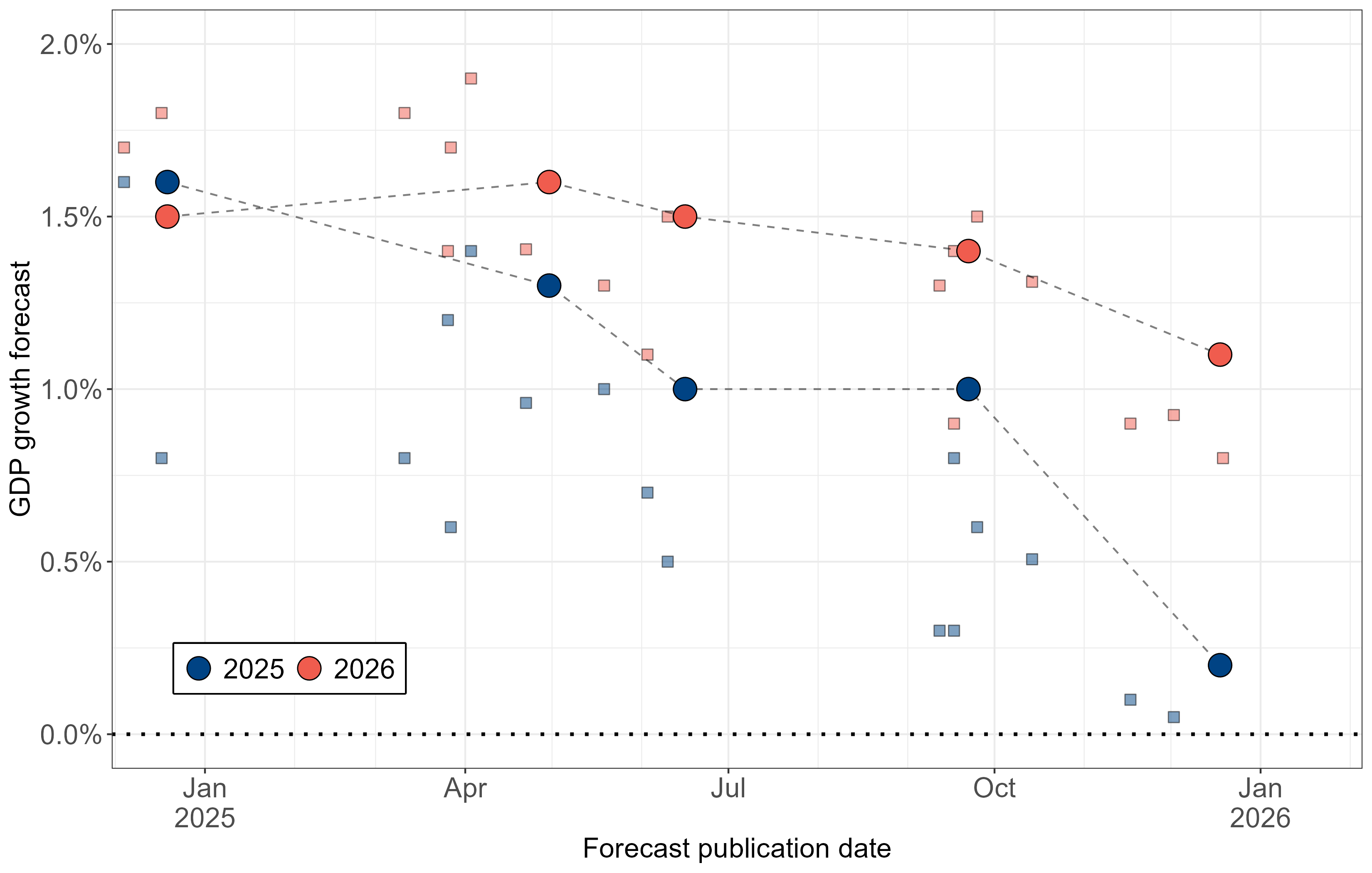
Notes: Ministry of Finance forecasts are represented by larger dots and connected by dashed lines. The other forecasting institutions included are: Bank of Finland, European Commission, IMF, OECD, Labore, Etla and PTT.
The figure separately identifies the Ministry of Finance forecasts for 2025 and 2026, on which the government relies when planning its fiscal policy. Over the course of the year, the Ministry of Finance forecasts for GDP growth in 2025 were more optimistic than most other forecasts published at roughly the same time, although the most recent forecast published in December 2025 no longer differed materially from the others. With respect to the growth forecast for 2026, no systematic difference relative to other forecasting institutions is discernible, at least not very clearly.
Figure 2.1.2 shows the contributions of different demand components to annual real GDP growth in 2021–2024 and, based on the Ministry of Finance forecast, in 2025–2028. In recent years, net exports and general government have contributed positively to GDP growth, whereas private consumption and, in particular, private investment have contracted in real terms.
The following subsections describe in more detail recent developments and the outlook for private consumption, investment, and exports and imports. Changes related to general government are discussed in greater detail in the chapter on the government’s fiscal policy (Chapter 6).
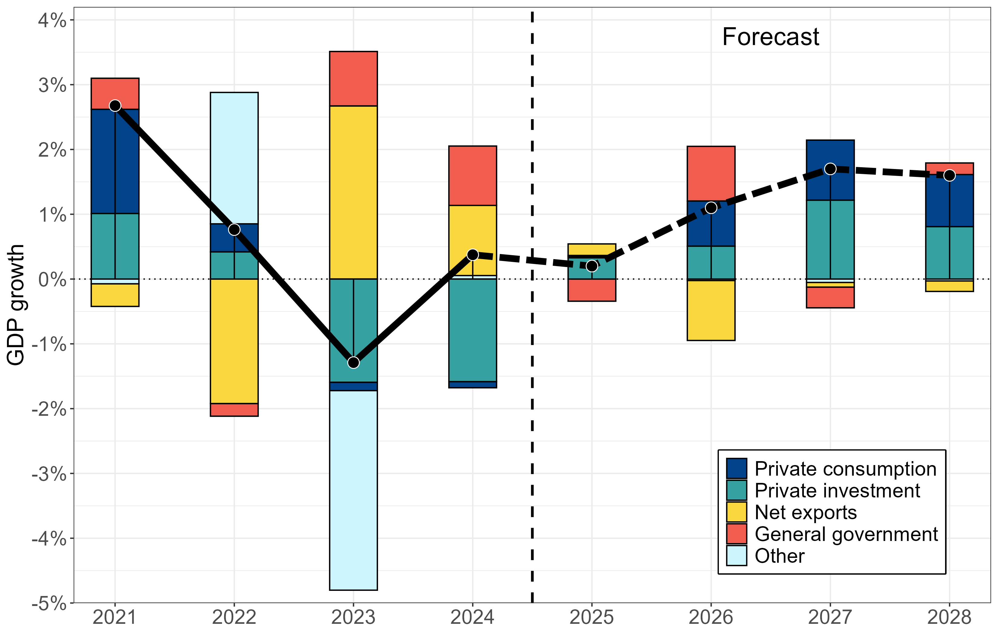
Source: Statistics Finland, Ministry of Finance (2025f).
Domestic consumption demand
Private consumption declined in real terms in 2023 and 2024. This is visible in Figure 2.1.2 as a small negative growth contribution from private consumption. The Ministry of Finance estimates that the volume of private consumption in 2025 remained at the previous year’s level (Ministry of Finance, 2025f), implying a zero growth contribution. At the same time, however, household disposable income has grown in recent years in both nominal and real terms.
Figure 2.1.3 depicts household saving, investment, net lending, and property income and expenditure relative to disposable income. By definition, gross saving is the difference between disposable income and individual consumption expenditure. Expressing this difference as a ratio to disposable income yields the gross savings rate.1 The figure shows that the gross savings rate began to rise during 2022. Households have thus been consuming a smaller share of their disposable income, which partly explains the subdued growth in private consumption in 2023–2025.
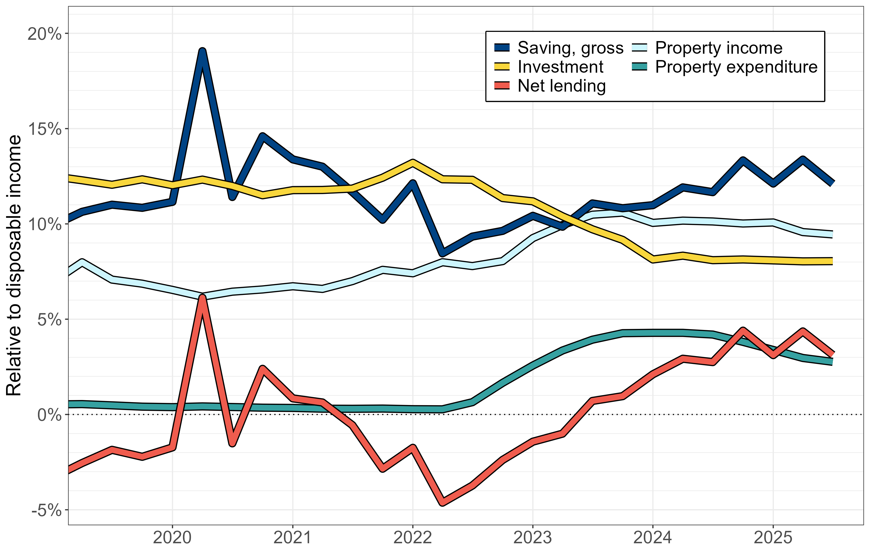
Source: Statistics Finland.
Figure 2.1.3 also shows that the ratio of household investment to disposable income (the investment rate) began to decline at the same time as the savings rate started to rise. This development has been reflected in the housing market, as household investment is predominantly directed towards housing.
The simultaneous increase in saving and decrease in investment have also marked a turning point in household indebtedness. The difference between the gross savings rate and the investment rate described above roughly corresponds to household net lending relative to disposable income. Figure 2.1.3 shows that, as the savings rate rose and the investment rate declined from 2022 onwards, household net lending has turned positive. In 2022, household net lending stood at approximately \(-\)4.5 billion euros, whereas by 2024 it was roughly the same amount in positive territory. The household debt-to-income ratio has accordingly begun to decline.2
These changes in household saving and investment behaviour have clearly reduced aggregate demand. The shift in the savings and investment rates coincided with the year 2022, when interest rates rose markedly from the previous near-zero level. The rise in interest rates may have altered household behaviour both by changing the attractiveness of saving or borrowing and by affecting household income and expenditure. The impact of higher interest rates is illustrated in Figure 2.1.3 particularly by the pronounced increase in property expenditure, which consists mainly of mortgage costs. On the other hand, household property income grew almost simultaneously. The increase in property income was, however, smaller than the increase in property expenditure.
The effects of higher interest rates vary considerably across households. For example, households whose wealth is predominantly in owner-occupied housing and who carry large mortgage debt are likely to have responded to higher interest rates differently from households with little or no debt who instead earn interest income. In addition to higher interest rates, many other factors may also underlie the changes in household saving behaviour, such as increased unemployment risk.
According to the Ministry of Finance forecast, private consumption will return to growth in 2026–2028 (Ministry of Finance, 2025f). In 2026, the volume of private consumption is forecast to grow by 1.4 per cent. Since the projected growth in consumption is nearly as rapid as the projected growth in household real disposable income (1.2 per cent), the household savings rate is not expected to change significantly. In subsequent forecast years, consumption growth would outpace income growth, implying a gradual decline in the savings rate from its current level.
Investment
The sharp contraction in private investment in 2023 and 2024 clearly weighed on aggregate output growth. In both years, private investment declined by approximately 8 per cent from the previous year. According to the Ministry of Finance forecast, private investment growth turned positive again in 2025, with investment increasing by 1.9 per cent compared to the previous year. The forecast projects that private investment growth will continue in the coming years, reaching its strongest pace in 2027, when growth is expected to be nearly 7 per cent. At that point, private investment growth would account for a significant share of aggregate output growth from the demand-side perspective (Figure 2.1.2).
The contraction in private investment in 2023 and 2024 was particularly linked to the collapse in residential construction. Figure 2.1.4 shows that the volume of new construction turned into a steep decline at the end of 2022, especially in the case of residential buildings. This turning point coincides with the rise in the general level of interest rates (see the following subsection). Based on the figure, the volume of new residential construction has roughly halved from its 2022 level.
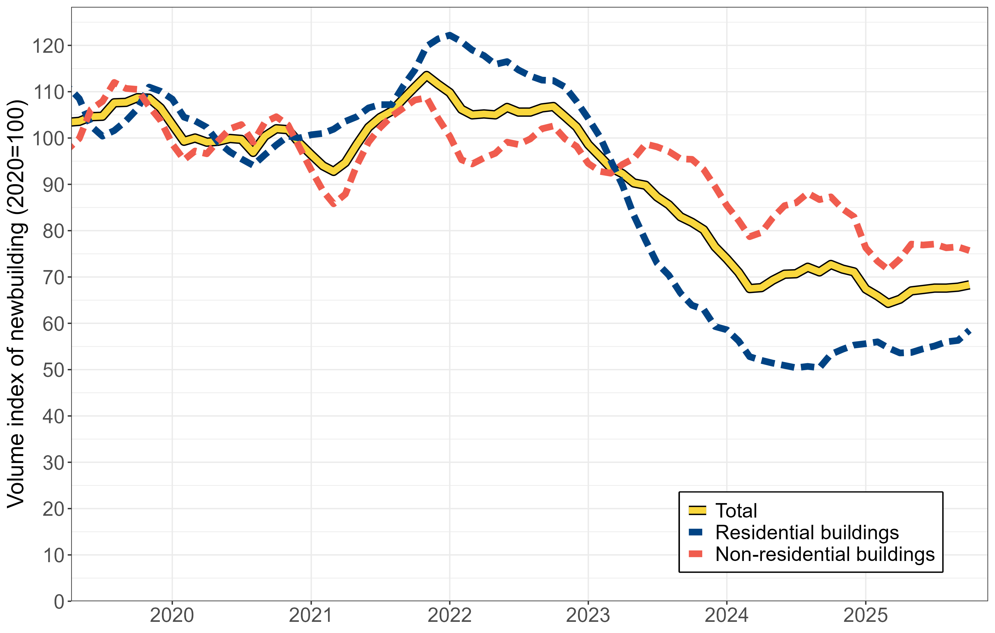
Source: Statistics Finland.
Residential construction includes renovation construction in addition to new construction. Although renovation construction has also declined, the decrease has been smaller than in new construction (Ministry of Finance, 2025d). Overall, residential construction investment has contracted by approximately one third from its 2022 level (Ministry of Finance, 2025f). This has undoubtedly had a major impact on the economy, as the share of residential construction in total investment was nearly one third in 2022.
According to the Ministry of Finance forecast, residential construction grew by 0.5 per cent in 2025. In 2026, the volume of residential construction is forecast to grow by 6 per cent, and in 2027 by 7 per cent.
Investment in machinery and equipment has not experienced a comparable collapse to that in construction. Investment in machinery and equipment declined by approximately 4 per cent in 2023 but grew by nearly 5 per cent the following year. In 2025, investment in machinery and equipment grew by around one per cent according to the Ministry of Finance forecast. In 2026, machinery and equipment investment will be boosted by the commencement of F-35 fighter jet deliveries, and total growth is forecast to be 13.5 per cent, partly on account of this. The fighter jet procurement is reflected in a sharp increase in public investment: public investment is forecast to rise by as much as 22 per cent in 2026, while private investment growth is forecast at 2.8 per cent (Ministry of Finance, 2025f). Investment growth is projected to exceed aggregate output growth over the entire forecast horizon.
Exports and imports
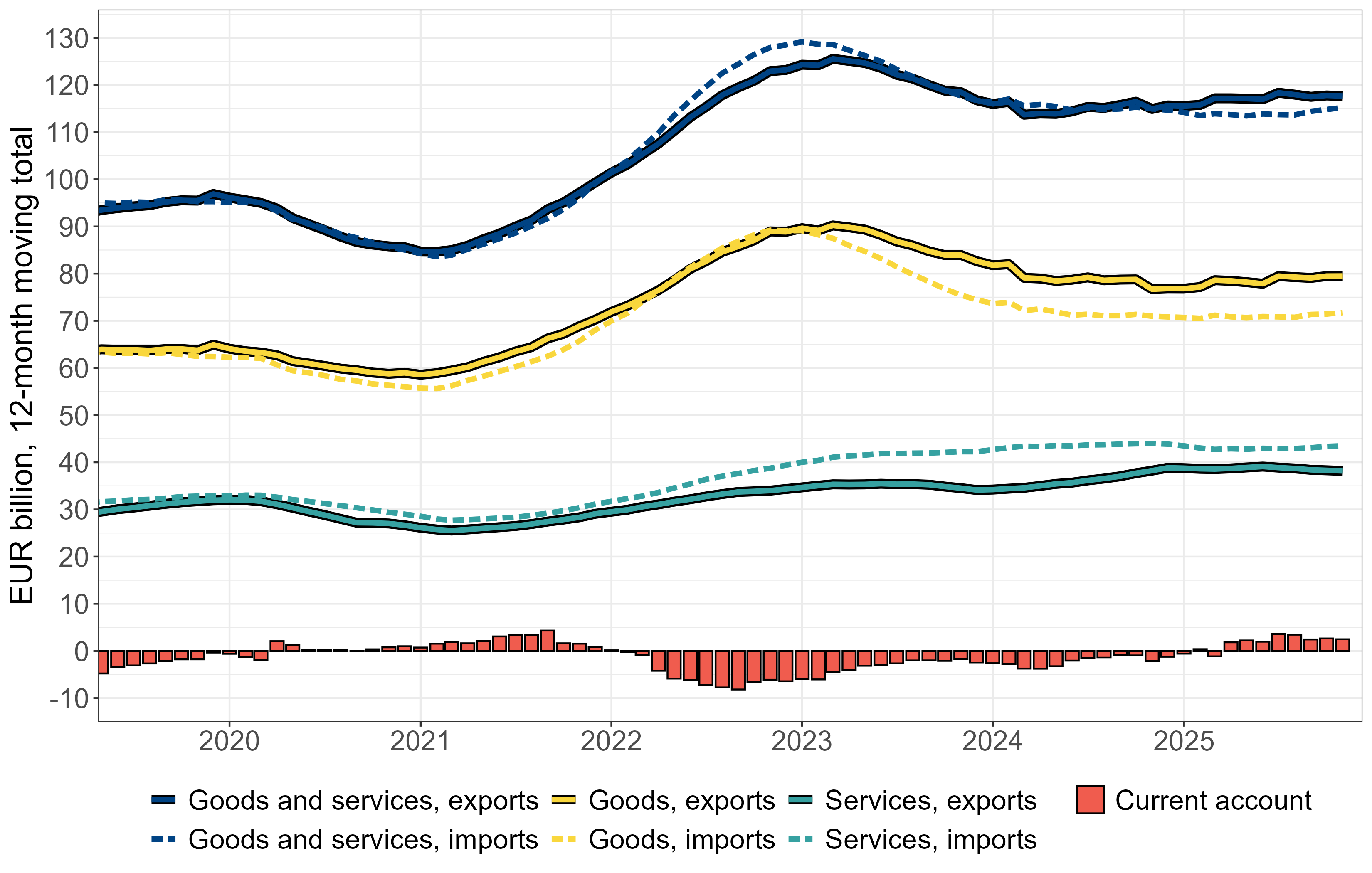
In recent years, net exports have contributed positively to GDP growth (Figure 2.1.2). However, the increase in net exports, particularly in 2023, was due to a contraction in imports rather than growth in exports, as both exports and imports declined from the previous year. Based on Figure 2.1.5, both exports and imports remain below their 2022 levels in current prices, but the contraction in imports has been considerably larger than that in exports.
Source: Statistics Finland.
In 2024, exports grew thanks to an increase in services exports. According to the Ministry of Finance forecast, the volume of exports grew by 1.8 per cent in 2024 and by 2.4 per cent in 2025. The volume of imports, by contrast, declined in 2024, with growth at \(-\)0.8 per cent. In 2025, the Ministry of Finance estimates that imports grew by 2 per cent (Ministry of Finance, 2025f).
When comparing changes in the volume of exports and imports with Figure 2.1.5, it should be noted that both export and import prices declined in 2024 and 2025. This means that the nominal developments shown in the figure do not directly reflect changes in export or import volumes. Finland’s terms of trade — the ratio of export prices to import prices — have been influenced in recent years in part by changes in energy prices. The terms of trade deteriorated in 2022, for example, as a result of the sharp rise in (imported) energy prices.
As exports have come to exceed imports, Finland’s current account also turned into surplus in 2025. A surplus on the current account means that the national economy as a whole is not accumulating debt to the rest of the world. The Ministry of Finance estimates that the current account surplus stood at 0.3 per cent of GDP in 2025, but forecasts that it will swing back into a roughly equivalent deficit in the near term. The forecast projects that both export and import volumes will grow in 2026–2028, but that import volumes will grow faster than exports (Ministry of Finance, 2025f).
Box 2.1. On US trade policy
The trade policy of the new US administration caused considerable turmoil in the spring of 2025. At the outset of Trump’s second term, tariffs were initially raised on products imported from Canada, Mexico and China, as well as on steel, aluminium and the automotive industry. At the same time, the administration was preparing a broader shift in trade policy. Uncertainty about the content of the new trade policy and the motives behind it pushed indices measuring policy uncertainty to historically high levels in the spring of 2025 (see e.g. Gensler et al. (2025)).
In early April 2025, the Trump administration launched so-called reciprocal tariffs, under which the tariffs imposed on imports from different countries would be determined by the size of the US trade deficit with each country. The stated minimum tariff level was, however, 10 per cent, applicable also to countries with which the United States runs a trade surplus. The proposed tariff levels were considerably higher than expected, and financial markets reacted strongly in the week following the announcement. The Trump administration soon decided on a 90-day pause on the reciprocal tariffs while maintaining the 10 per cent minimum tariff level. A brief trade-war-like situation also developed between China and the United States, with both sides raising trade barriers in turn. Subsequently, however, tariffs between the two countries also settled at lower levels.
These so-called reciprocal tariffs were ultimately applied in the late summer. Following the launch of the new tariff policy, the US administration has, however, agreed on lower import tariffs with several trading partners. These agreements may have stipulated lower tariffs conditional on certain other policy objectives being advanced. For example, the agreement with the EU, which set a tariff ceiling of 15 per cent with some exceptions, stipulated that the EU would not levy tariffs on US products and that EU member states would purchase large quantities of liquefied natural gas from the United States.
Despite these trade agreements, there remain uncertainties regarding the stability of the tariffs. First, there is significant legal uncertainty surrounding the implementation of tariff policy. Under US law, the authority to regulate foreign trade and impose tariffs rests primarily with Congress, not the President. The Trump administration has justified its sweeping tariff increases by invoking exception statutes previously enacted by Congress that grant the President powers to intervene in trade on grounds such as national security or unfair trade practices. The matter is pending before the Supreme Court, but no binding precedent has yet been established. Due to the slow pace of legal proceedings, the tariffs remain in force and payable even though their legality continues to be contested.
The Trump administration has also demonstrated a willingness to deviate from established trade agreements and to use tariff threats as an aggressive negotiating tactic. The most recent example is the diplomatic dispute over the status of Greenland, which threatened to jeopardise the trade agreement negotiated with the EU. The United States threatened to impose an additional 10 per cent tariff from February 2026 on countries — Finland included — deemed to be obstructing its objectives. The situation, however, appeared to dissipate as quickly as it arose, as only a few days later Trump announced the withdrawal of the immediate tariff threat, reportedly following the emergence of a preliminary understanding on an Arctic agreement. This episode underscores the unpredictability of Trump’s trade policy: tariff policy can change with a single social media post.
As a consequence of Trump’s second-term trade policy, US tariff levels in 2025 were higher than at any point since the 1940s. At the beginning of 2026, US consumers were estimated to face an average effective import tariff of approximately 17 per cent (Yale Budget Lab, 2026).
Import tariffs are fundamentally a tax that creates a wedge between the price paid by the domestic buyer and the price received by the foreign seller. As such, they distort the global division of labour and lead to a less efficient allocation of economic resources than would prevail in the absence of tariffs. For the country imposing the tariffs, they constitute a negative supply shock; for other countries, they are primarily a negative demand shock. However, in a situation where countries face tariffs of different magnitudes, domestic industry may benefit from its own country’s import tariffs. On the other hand, with globalisation, the economy and its production chains have become increasingly complex, and even the industry of the tariff-imposing country is readily harmed by tariffs if it uses imported intermediate inputs in its production.
In addition to the effects described above, the uncertainty associated with trade policy is also likely to reduce investment. One mechanism is related to the fact that investments are often irreversible. If the profitability of an investment project depends on trade policy and there is substantial uncertainty about future policy, it may be worthwhile to defer the investment decision until the uncertainty clears. There is also empirical evidence of the negative impact of trade policy uncertainty on investment; see for example Caldara et al. (2020).
As a small open economy, Finland is exposed to uncertainty related to trade policy. Although the majority of Finland’s foreign trade takes place within the EU internal market, the United States accounted for approximately 10 per cent of Finland’s goods exports in 2024, with the value of goods exports to the United States amounting to approximately 8.1 billion euros. Finland’s trade balance with the United States was also strongly in surplus, with the value of goods imports standing at approximately 3 billion euros in 2024.a
The economic impact of the tariffs is mitigated by the fact that services are excluded from tariffs. Finland’s services exports to the United States amounted to approximately 6.1 billion euros in 2024, and services imports to approximately 5 billion euros.
The effects of US tariff policy on the Finnish economy have been assessed ex ante by, among others, Juvonen et al. (2024), Ali-Yrkkö (2025) and Silvo and Juvonen (2025). Assessing the effects ex ante is, however, challenging, as every modelling exercise must be based on certain assumptions about the eventual conditions of the trade policy landscape and the durability of higher tariffs. The models also differ in terms of which effects they aim to capture. The above-mentioned assessments assumed tariff rates of 10–25 per cent on Finnish exports. The estimated GDP impact in these assessments ranges roughly from \(-\)0.5 per cent to \(-\)1.6 per cent.
2.2 Inflation and interest rates
Inflation
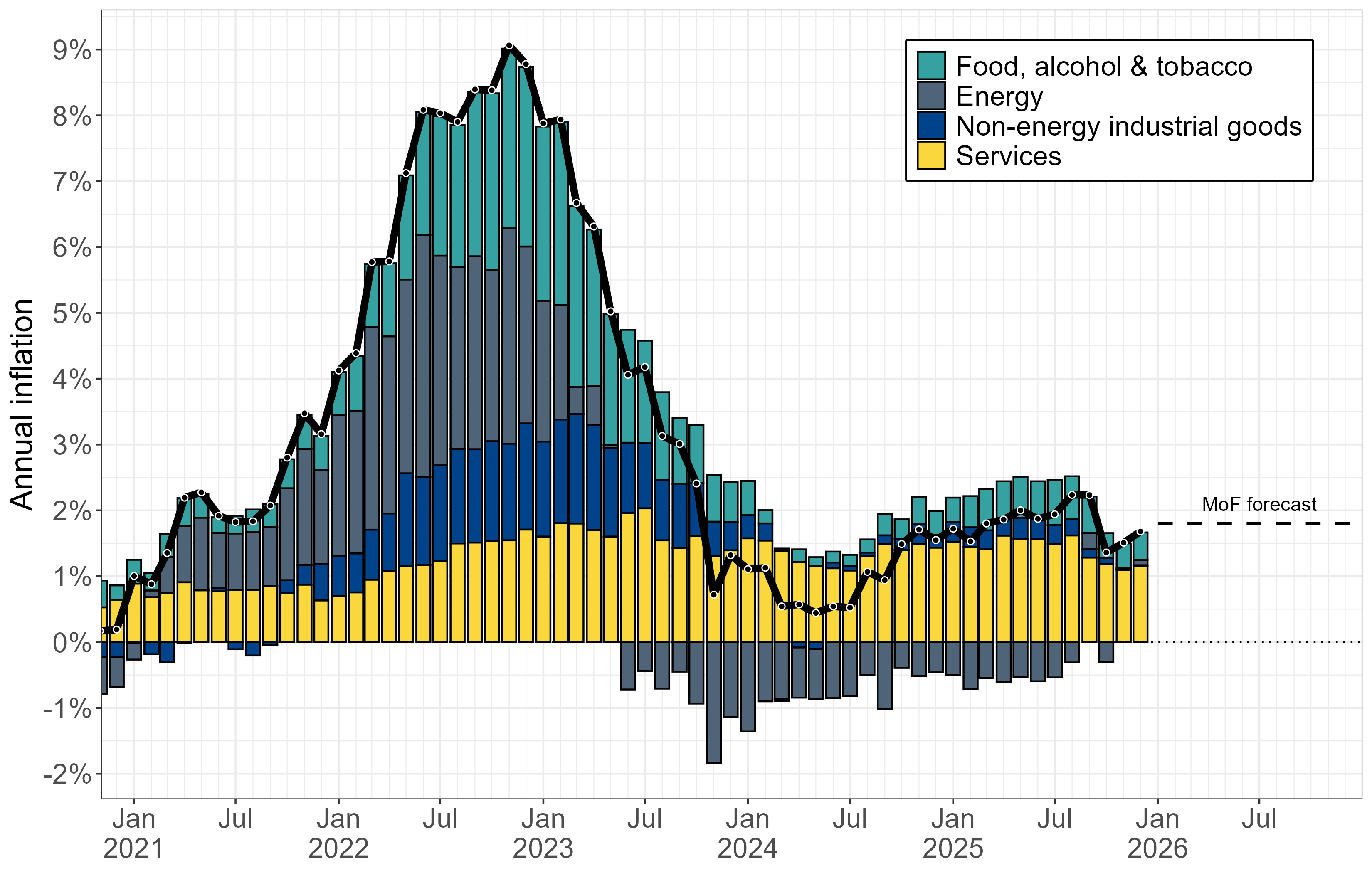
Inflation as measured by the Harmonised Index of Consumer Prices (HICP), which captures inflation excluding the impact of interest expenses, stood at approximately 1.8 per cent in 2025. According to the decomposition in Figure 2.2.1, the main upward driver of inflation has been the rise in services prices. Energy prices have, by contrast, continued to slightly dampen inflation. The Ministry of Finance forecasts a similar inflationary path going forward: the HICP is projected to rise by 1.8 per cent also in 2026 and 2027 (Ministry of Finance, 2025f).
Source: Statistics Finland, Ministry of Finance (2025f).
Notes: The bars represent the contributions of different consumption categories to overall inflation,
shown by the black line. The dashed line represents the Ministry of Finance forecast for the full year
2026.
Interest rate developments
During 2025, the ECB lowered its key policy rate from 3 per cent at the beginning of the year to 2 per cent. The last rate change took place in June. Euro area inflation has recently been close to the 2 per cent target, so there is no immediate pressure to ease or tighten monetary policy in this regard. Based on market interest rates in January 2026, the next rate change is expected to be a rate increase rather than a rate cut.
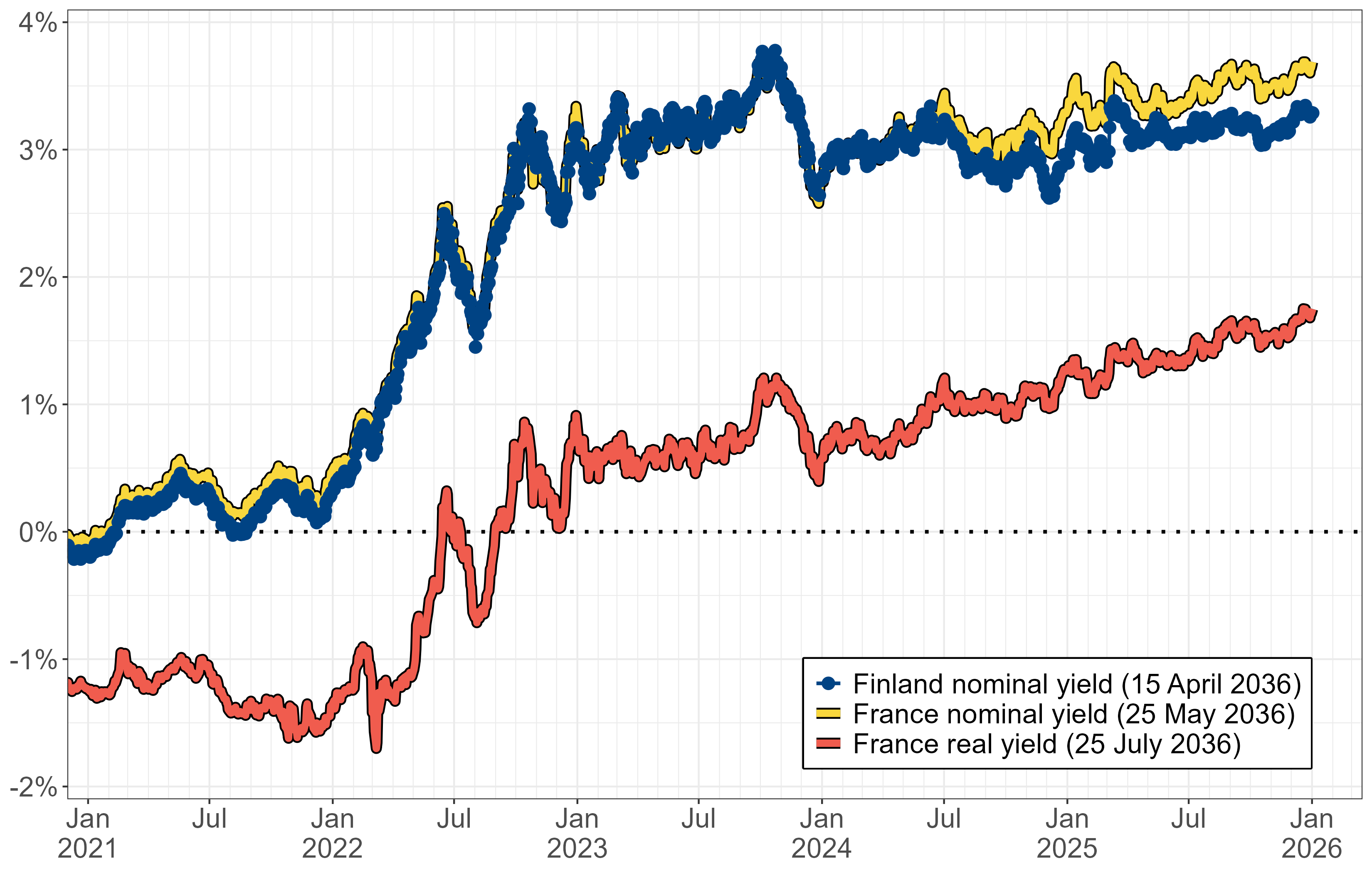
Figure 2.2.2 shows the yield developments of selected Finnish and French government bonds maturing in 2036 over the past five years. For France, the figure depicts the development of both the nominal and the real yield. The real interest rate refers to the nominal interest rate adjusted for inflation. It is a more important price than the nominal rate when considering, for example, the economic incentive to save or the burden that public debt servicing places on public finances. The real yield is derived from the secondary market prices of inflation-linked French government bonds indexed to the euro area consumer price index. For Finland, the figure shows only the yield on a nominal government bond of corresponding maturity, as Finland has not issued inflation-linked government bonds.
Source: Bank of Finland, Agence France Trésor (Bloomberg).
Notes: The maturity date of the bond is shown in parentheses. The French real yield is for an OAT€i bond
indexed to the euro area Harmonised Index of Consumer Prices.
Although a small gap has opened between Finnish and French nominal government bond yields over the past year, the overall development of yields has been sufficiently similar to justify the assumption that the real yield on French government bonds is fairly close to the real interest rate that investors would, in expected value terms, require to lend to the Finnish government.
The real yield on French government bonds rose slightly during 2025, standing at approximately 1.5 per cent at year-end. For Finland, the real yield can be estimated to have risen somewhat less over the same period, as the nominal yield on French government bonds has risen above that of Finnish bonds. In any case, the substantial rise in the real interest rate that occurred in 2022 appears to have been permanent, at least for the time being. This makes the servicing of public debt considerably more expensive than before (see EPC (2024), Chapter 2.4).
2.3 Labour markets
Unemployment
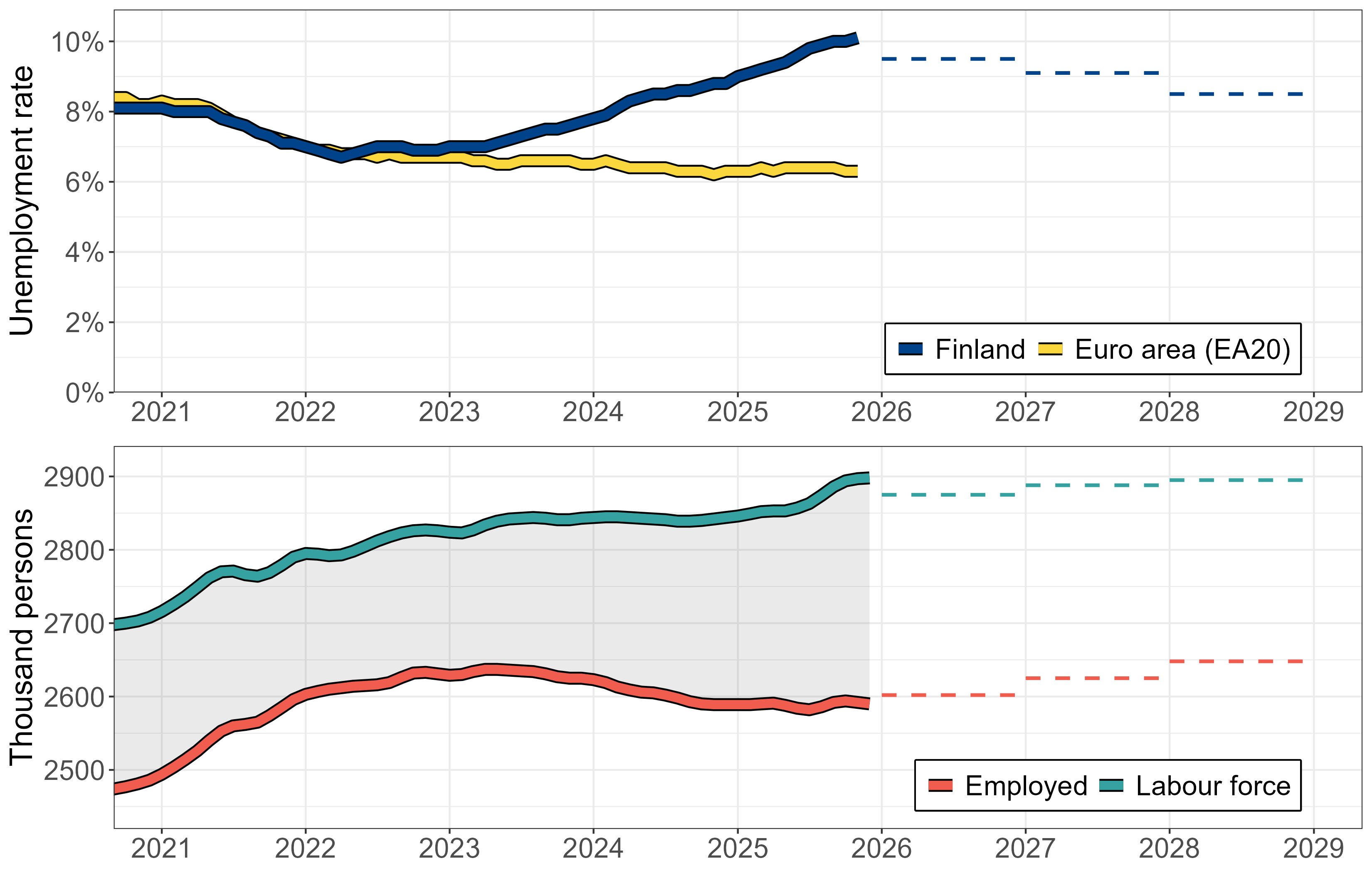
The unemployment rate based on Statistics Finland’s Labour Force Survey has been rising in Finland since 2022. In 2022, the unemployment rate in the 15–74 age group was 6.8 per cent, compared to 9.7 per cent in 2025. The upper panel of Figure 2.3.1 compares the trend in the unemployment rate in Finland and the euro area, based on Eurostat data. In 2021 and 2022, unemployment rate developments were still very similar, but since then Finland’s unemployment rate has embarked on an upward trajectory while the euro area rate has continued on a gently declining trend. According to the Ministry of Finance forecast, Finland’s unemployment rate will remain elevated in the near term, still standing at 9.5 per cent in 2026 (Ministry of Finance, 2025f). The Ministry of Finance forecasts for the different years are shown by dashed lines in the figure.
Source: Eurostat, Statistics Finland, Ministry of Finance (2025f).
Notes: Ministry of Finance forecasts for the full years 2025–2028 are shown by dashed lines.
The lower panel of Figure 2.3.1 shows separately the trend in the number of employed persons and in the labour force in Finland over the same period, based on Statistics Finland’s Labour Force Survey. The unemployment rate is the difference between the labour force and the number of employed persons (the number of unemployed) divided by the labour force. The figure shows that although the number of employed persons has declined from its 2023 level, the recent increase in unemployment largely reflects growth in the labour force. The labour force grew fairly rapidly, particularly towards the end of 2025. At the same time, the unemployment rate rose even though the number of employed persons changed only marginally. According to the Labour Force Survey, the number of unemployed persons in 2025 was 278 thousand on an annual basis, which is 74 thousand more than in 2023. Over the same period, the labour force grew by 36 thousand and the number of employed persons declined by 38 thousand.
Employment rate
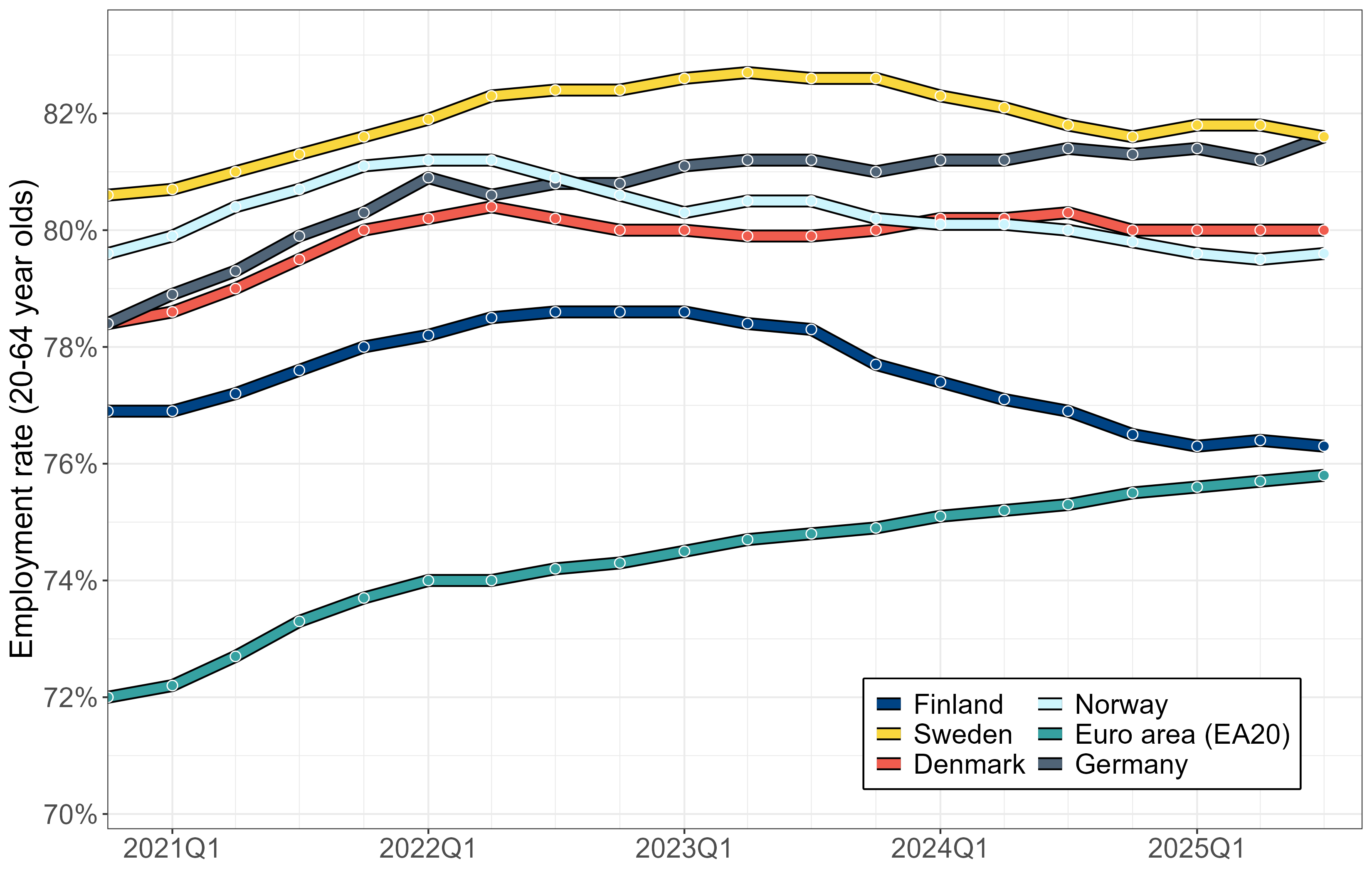
Figure 2.3.2 shows employment rate developments in the 20–64 age group in selected countries, based on Eurostat data. According to Statistics Finland’s Labour Force Survey, the employment rate in this age group was 76 per cent in Finland in 2025, approximately 2 percentage points lower than in 2022, when the employment rate peaked. Although the employment rate in 2025 was lower than in preceding years, the figure suggests that the declining trend in the employment rate appears to have levelled off during 2025.
Source: Eurostat.
Among the countries shown in Figure 2.3.2, the employment rate has also declined slightly in Sweden and Norway, whereas in Denmark and Germany it has remained very stable over the same period. The euro area employment rate has grown steadily and is now close to Finland’s level.
Job vacancies and labour market tightness
The Beveridge curve describes the relationship between unemployment and job vacancies. (The vacancy rate shown in the figure is the ratio of vacancies to the labour force.) There is typically a negative relationship between the two: during periods of high unemployment, vacancies are few, which is characteristic of a downturn. Conversely, during periods of low unemployment, vacancies are plentiful, which is typical of a boom.
Figure 2.3.3 shows how the unemployment rate and the vacancy rate in Finland have evolved in relation to each other. The differently coloured Beveridge curves in the figure represent periods during which the relationship between unemployment and vacancies has remained relatively stable. These Beveridge curves have, however, shifted outwards when more recent time periods are examined compared to preceding decades. This outward shift means that a given number of vacancies relative to the labour force is typically associated with a higher unemployment rate than before.
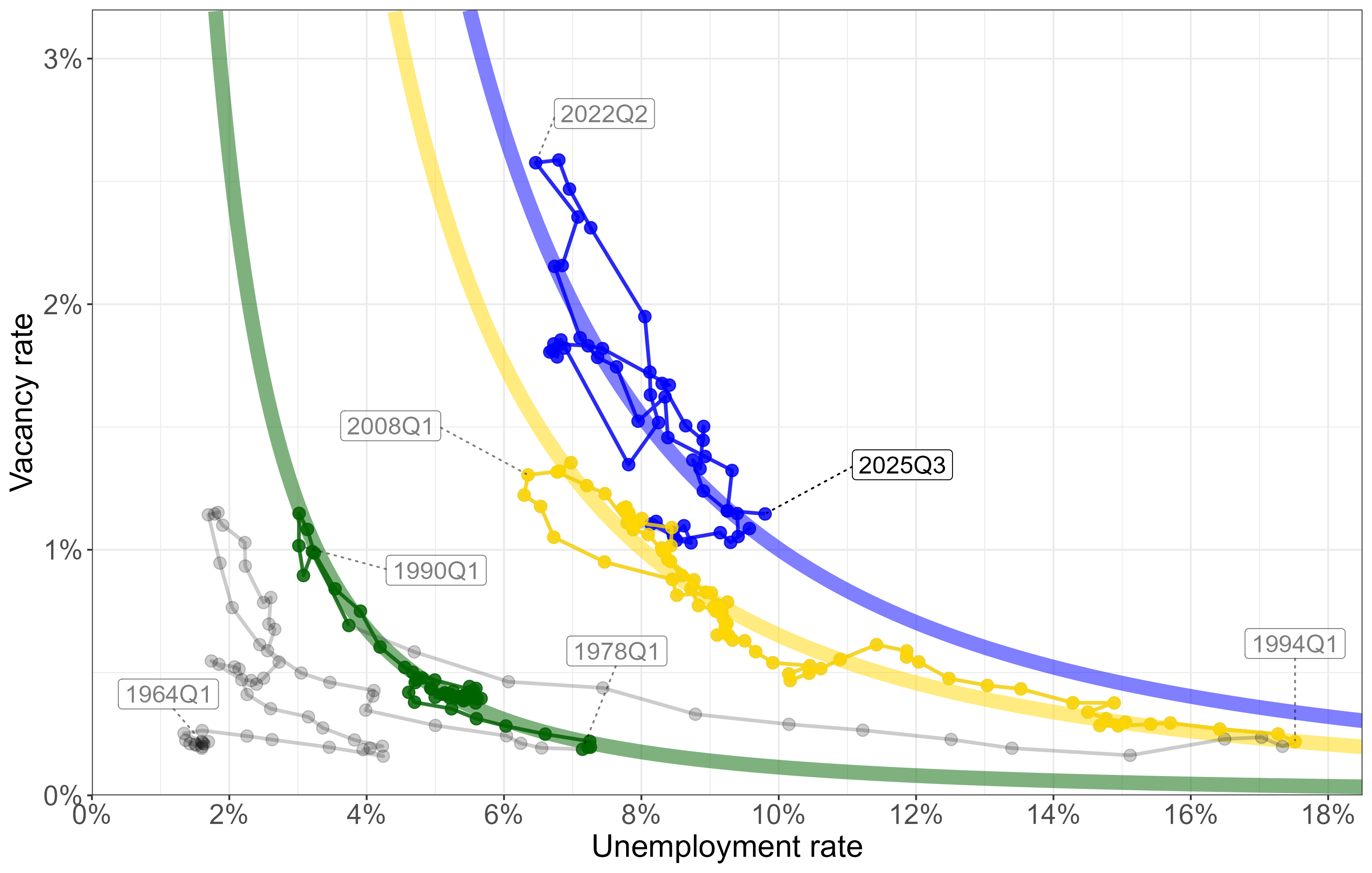
Source: Gäddnäs and Keränen (2023), updated with more recent Eurostat data.
Notes: The coloured Beveridge curves represent the average positions of the curves in 1978–1990 (green curve),
1994–2012 (yellow curve) and 2013– (blue curve).
Examining developments in recent years reveals that the tight labour market of 2022 has, by 2025, deteriorated markedly from the perspective of workers. The approximately three-percentage-point increase in the unemployment rate from its 2022 level has been accompanied by a decline in the vacancy rate from approximately 2.5 per cent to slightly above 1 per cent. This development broadly follows the blue Beveridge curve in the figure, suggesting that it reflects a standard cyclical weakening.
2.4 Council views
Economic activity has remained subdued throughout the government term, as measured by both employment and GDP growth. At the beginning of the government term, the weak performance was driven in particular by the rapid decline in housing construction that began as early as 2022.
The pronounced volatility of construction is more broadly harmful to the economy. It amplifies cyclical fluctuations and leads to an inefficient use of resources, as a significant share of construction sector workers are periodically without work. Going forward, efforts should be made to smooth construction volatility, for example by scheduling public construction projects more countercyclically and by promoting steadier private construction activity. This could be supported, for example, by ensuring a more even disposal of city-owned plots for construction over the business cycle and by allowing plot prices to adjust flexibly in line with demand.
The rise in the household savings rate has also weighed on economic growth in recent years. It has reduced domestic demand at a time when output is constrained to some extent by insufficient aggregate demand relative to productive capacity. The weak cyclical situation has also likely amplified the short-term adverse effects of the government’s consolidation measures, described in Chapter 6, on output and employment through the aggregate demand channel.
The increase in the household savings rate is not necessarily detrimental to longer-term economic development. It has already turned Finland’s current account from a small deficit into a small surplus, meaning that the Finnish economy as a whole is saving. This can be seen as a natural way of preparing for foreseeable expenditure pressures, such as the growth in care expenditure associated with population ageing and the need to increase defence spending in response to the deteriorated security environment.
Output and employment can grow through exports rather than domestic demand. However, the reallocation of labour from the domestic market sector to export industries takes time. Improved employment through stronger export demand also requires sufficiently strong cost competitiveness.
The unemployment rate has risen to a very high level compared to recent years. At the same time, however, the labour force has grown markedly. The growth of the labour force is a positive development from the perspective of future economic growth. It means that labour shortages will not immediately become a constraint on growth as the economy recovers.
3 Finances of the wellbeing services counties
In our previous annual report, we described the funding model for the wellbeing services counties (WSCs), the state of their finances in 2023 and 2024, and the challenges arising from the obligation to cover deficits. In this chapter, we assess the financial situation of the WSCs in 2025 and their near-term outlook, based on the data reported by the counties in early autumn 2025. In addition, we examine the assessment of service need, which is central to the funding of the counties and the problems associated with its application. Finally, we assess the savings targets set by the government for the WSCs and progress towards meeting them.
The wellbeing services counties reported their 2025 financial statement estimates at the end of January 2026. Based on the updated data, the combined 2025 result at the national level would be better than the forecast data suggested.3 The update does not materially change the overall picture of WSC finances presented in this chapter, but the divergence between counties appears to be intensifying.
3.1 Financial situation of the wellbeing services counties in 2025
After two years of significant deficits, the combined finances of the wellbeing services counties are turning to a slight surplus in 2025. Based on the financial statement forecasts, the WSCs would have a combined surplus of approximately EUR 200 million in 2025. This considerable improvement in the financial situation is primarily explained by the EUR 1.4 billion ex-post adjustment added to funding in 2025 and by expenditure growth remaining at a moderate level of approximately 3 per cent.
Despite the surplus result in 2025, the wellbeing services counties have a total of EUR 2.2 billion in accumulated deficit. The accumulated deficit is primarily attributable to the rapid growth in expenditure in 2023.4 Although expenditure growth slowed markedly already in 2024, the finances of the WSCs were still significantly in deficit that year, as the level of WSC funding is adjusted through the ex-post adjustment to match realised expenditure only with a two-year lag. At the national level, funding in 2024 was approximately EUR 400 million, or approximately 2 per cent, less than realised expenditure in 2023.
The purpose of the ex-post adjustment is to ensure that realised expenditure does not diverge from funding at the national level and that the WSCs thereby have the means to carry out their assigned tasks.5 However, the restoration of balance in WSC finances as measured by the deficit alone is not sufficient: under current legislation, the deficit accumulated in 2023 and thereafter must be covered by corresponding surpluses by the end of 2026.6
Financial situation by county
Although the combined finances of the WSCs are turning to a slight surplus, the financial divergence between counties is continuing and intensifying. Despite the moderate growth in expenditure, ten counties remain in deficit in 2025. The ex-post adjustment added to funding in 2025 was allocated to the counties in proportion to their imputed funding, not on the basis of county-specific deficits. This has contributed to the divergence in the financial situation across counties. Figure 3.1.1 shows the accumulated deficit (or, in the case of Helsinki, the accumulated surplus) of each WSC over 2023–2025, relative to county-specific central government funding in 2026. In order to cover their accumulated deficits by the end of 2026, the counties would need to generate surpluses corresponding to the shares of 2026 funding shown in the figure.
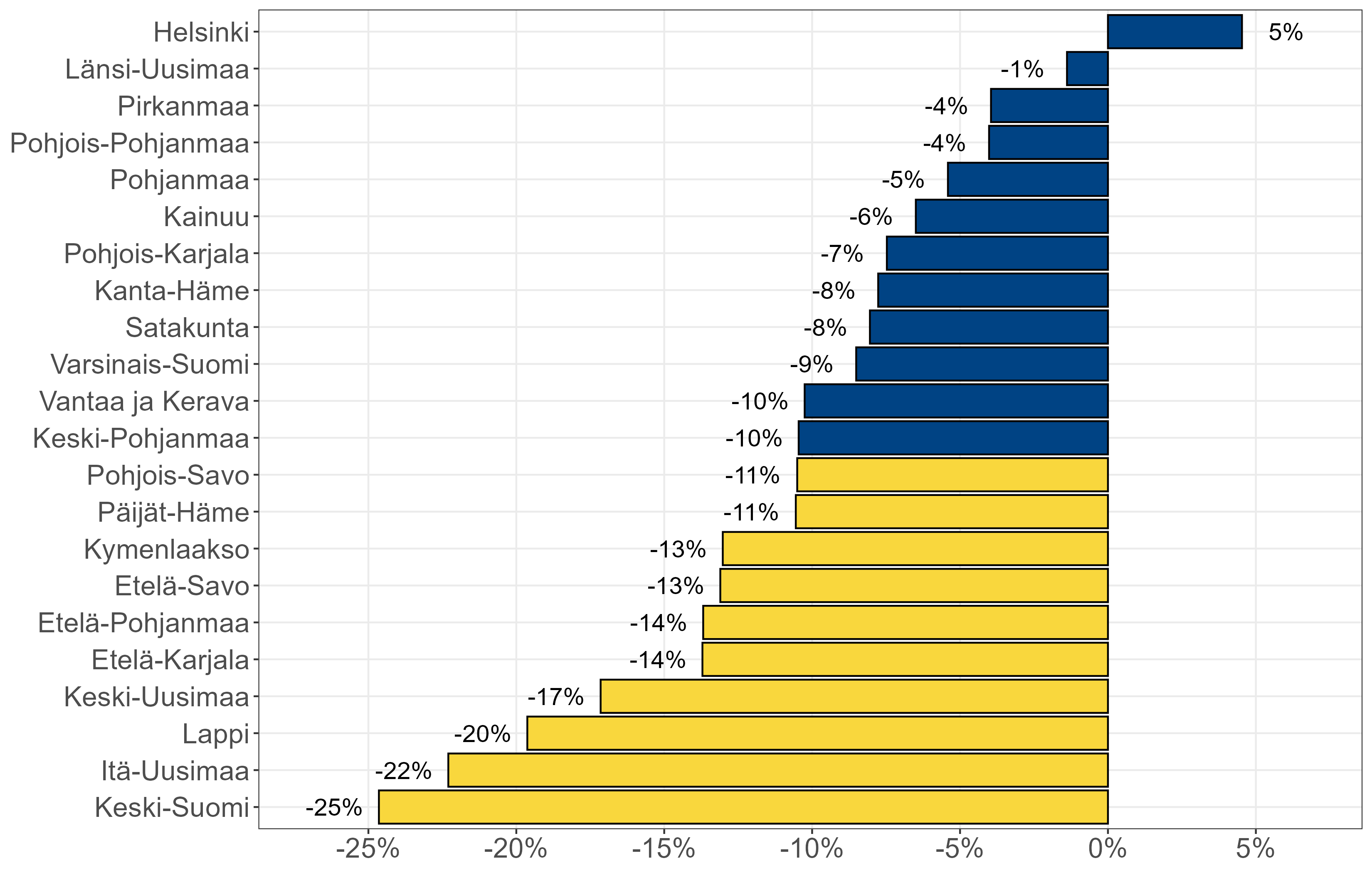
Counties marked in blue had a surplus in 2025 based on the financial statement forecasts, while counties marked in yellow were in deficit in 2025. Source: State Treasury, Ministry of Finance, Council’s calculations.
The figure shows that there are significant differences in the financial situation across counties. The City of Helsinki has the strongest financial position. At the end of 2025, it has approximately EUR 140 million in accumulated surplus, corresponding to a surplus of approximately 5 per cent relative to Helsinki’s 2026 funding.
Based on the financial statement forecasts, 11 wellbeing services counties are on track to move from deficit into surplus in 2025. The blue bars in Figure 3.1.1 show, however, that the 2025 surplus is not sufficient in any of these counties (excluding Helsinki) to cover the deficit accumulated in 2023 and 2024. Taking into account the projected 2025 surplus, the remaining deficit to be covered in these counties ranges from 1 to 10 per cent relative to 2026 central government funding. In euro terms, the combined accumulated deficit of these counties stands at EUR 875 million at the end of 2025.
Despite the moderate growth in expenditure, ten counties remain in deficit in 2025 according to the financial statement forecasts (yellow bars in Figure 3.1.1). The combined deficit of these counties over 2023–2025 ranges from 11 to 25 per cent relative to 2026 funding. In euro terms, this group’s accumulated deficit over 2023–2025 totals approximately EUR 1.5 billion. The weakest financial positions are in Keski-Suomi, Itä-Uusimaa and Lappi, all of which have accumulated deficits exceeding 20 per cent relative to their 2026 funding.
Reasons for the financial divergence
The imbalance between funding and expenditure became very significant for several counties already in 2023, as expenditure growth varied between 4 and 17 per cent across counties. Reasons for the differences in expenditure growth across counties included, among others, differences in the initial conditions regarding the integration of services and finances. The baseline year 2022 expenditure data reported by the municipalities contained deficiencies due to municipalities’ incentives to under-budget health and social care expenditure and due to the impact of the COVID-19 pandemic on service provision. In addition, some counties initiated fiscal consolidation already in 2023.
The national level of funding is adjusted annually by the WSC price index, by the estimated growth in service need, by changes in funding corresponding to changes in statutory tasks, and by the ex-post adjustment. The county-specific allocation of funding is also updated annually to reflect changes in population structure, county-specific health and social care service need, and other factors determining the level of funding. In addition, funding is affected by county-specific transitional equalisation additions and deductions. Figure 3.1.2 shows the development of funding over 2022–2026 by county, broken down into changes in imputed funding, the ex-post adjustment, and transitional equalisations.
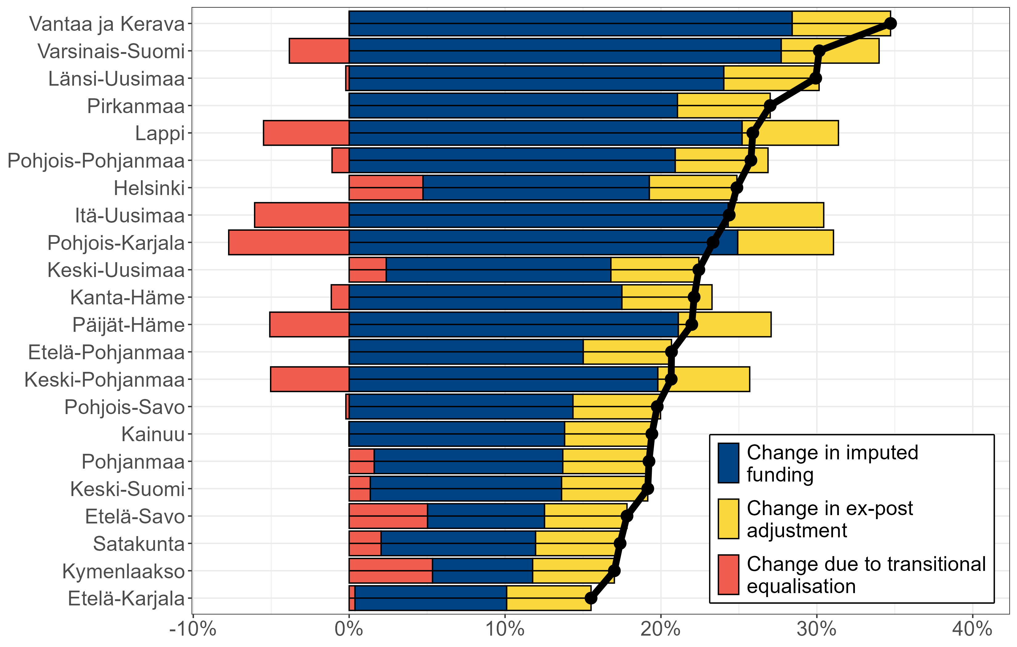
Black dots represent the total change in funding over 2022–2026. Source: State Treasury, Ministry of Finance, Council’s calculations.
At the national level, WSC funding in 2026 is nominally 24 per cent higher than the amount that municipalities reported spending on the provision of corresponding services in 2022. By county, funding has increased by 16 to 35 per cent compared to the 2022 expenditure of the municipalities in each county’s area. County-specific changes in imputed funding are primarily explained by changes in population and estimated service need.
Figure 3.1.2 also shows the share of the 2025 and 2026 ex-post adjustments in funding. The ex-post adjustment to funding does not reflect county-specific deficits but only the combined expenditure developments of all counties. The figure shows that the funding increase through the ex-post adjustment is roughly proportional for all counties. As a result, Helsinki, which was the only county to record a slight surplus in 2023 and 2024, receives a total of EUR 290 million through the ex-post adjustment in 2025 and 2026. On the other hand, the ex-post adjustment covers only approximately 60 per cent of the 2023 and 2024 deficits of Keski-Suomi, Lappi and Itä-Uusimaa, which are in the weakest financial position. For these counties, the ex-post adjustment falls EUR 225 million short of their combined accumulated deficit.
3.2 Extension of the deficit-covering period
In our previous annual report, we recommended granting additional time for the deficit-covering period, so that counties could spread their expenditure adjustments more evenly over several years. In our assessment, the obligation under existing legislation to cover deficits by the end of 2026 would force many counties first to make very substantial spending cuts, after which they would have the opportunity to increase expenditure rapidly.7
Covering the deficits by the end of 2026 would mean that the WSCs would need to cut their expenditure at the national level by an estimated 4 per cent in nominal terms in 2026 compared to 2025. Figure 3.2.1 shows the county-specific maximum change in expenditure that would allow each county to cover the accumulated deficit shown in Figure 3.1.1 by the end of 2026.
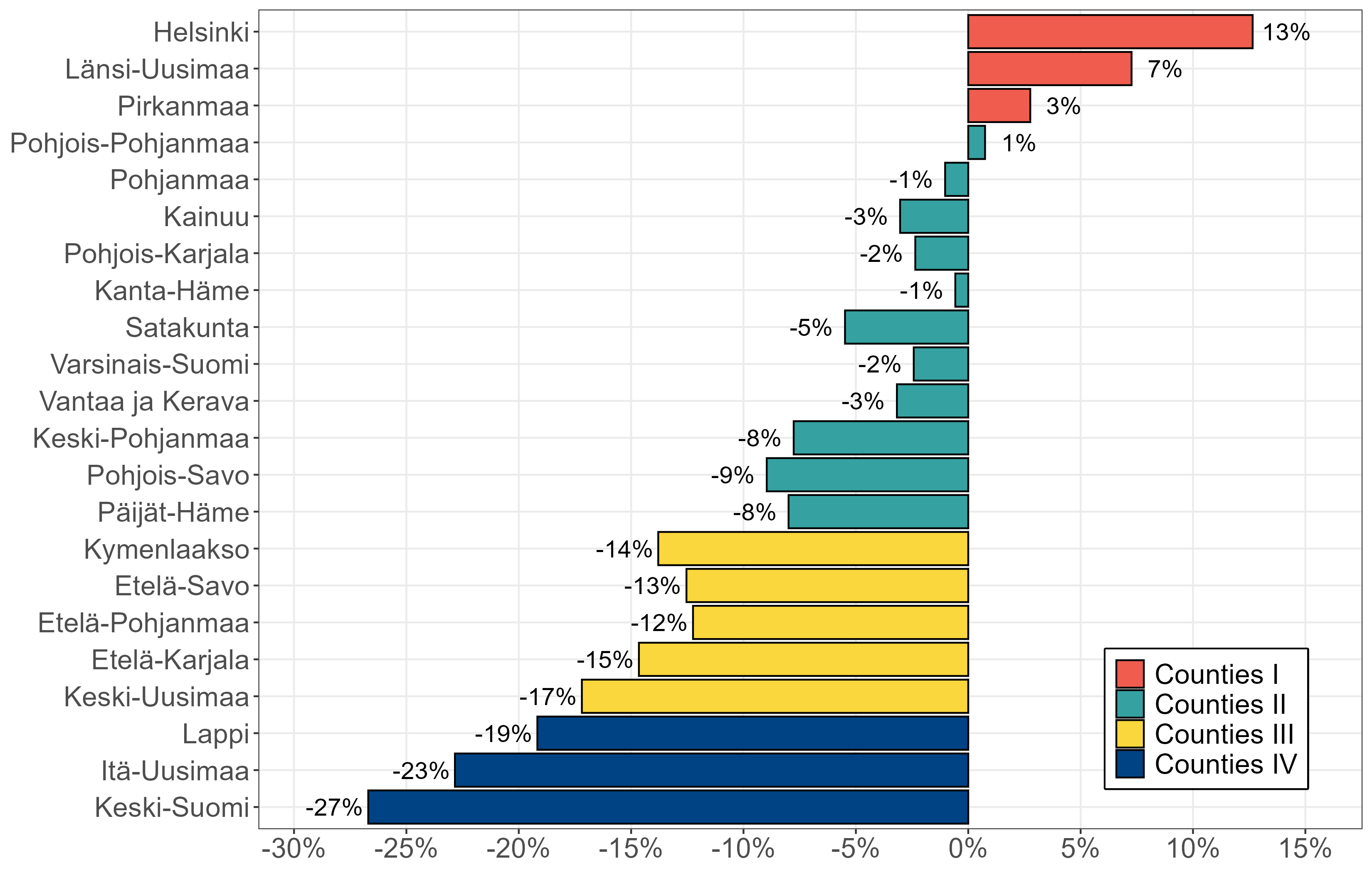
The bars represent the county-specific maximum change in expenditure in 2026 that would allow counties to cover their accumulated deficit by the end of 2026. Counties are ordered according to the accumulated deficit shown in Figure 3.1.1. Classification of counties: I: Counties that are likely to cover their deficits during 2026, and Helsinki. II: Counties with an accumulated deficit of 4–11% relative to 2026 funding. III: Counties with an accumulated deficit of 13–17% relative to 2026 funding. IV: Counties with an accumulated deficit exceeding 20% relative to 2026 funding. Source: State Treasury, Ministry of Finance, Council’s calculations.
The figure shows that for the majority of counties, covering deficits during 2026 would require nominal cuts to expenditure. The required cuts range from 1 to 27 per cent. A few counties would be able to cover their deficits even if expenditure were to increase in nominal terms in 2026. In the case of Helsinki, the maximum change in expenditure shown in the figure would mean that Helsinki would draw down its accumulated surplus and its finances would be in balance at the end of 2026. The figure shows that the scale of the required consolidation or possible expenditure growth does not depend directly on the amount of accumulated deficit at the end of 2025 shown in Figure 3.1.1. The county-specific consolidation requirement is also affected by the timing of consolidation measures already undertaken and by the development of funding.
The government submitted a legislative proposal (HE 189/2025) in late 2025, proposing a temporary amendment to the legislation governing the covering of deficits. Under the proposal, the Ministry of Finance could, upon application by a county, grant an extension of one or two years for covering deficits. Counties could thereby spread the required spending cuts over a maximum of three years.
In the Ministry of Finance forecast, the annual growth in WSC expenditure is estimated at approximately 4 per cent in 2026–2028, taking into account the growth in wages in the health and social care sector that exceeds the general increase in the level of earnings.8 The forecast is by nature a pressure calculation, meaning that it does not assume significant consolidation measures by the counties themselves. Figure 3.2.2 shows the expenditure development consistent with the Ministry of Finance forecast for 2026–2028, as well as the development of central government funding in 2028–2030 if expenditure were to develop as forecast. The figure shows that if the Ministry of Finance forecast were to materialise, the WSCs would be only marginally in surplus in 2026–2027 and slightly in deficit again in 2028. In aggregate, the WSCs would still have approximately EUR 1.6 billion in accumulated deficit at the end of 2028.
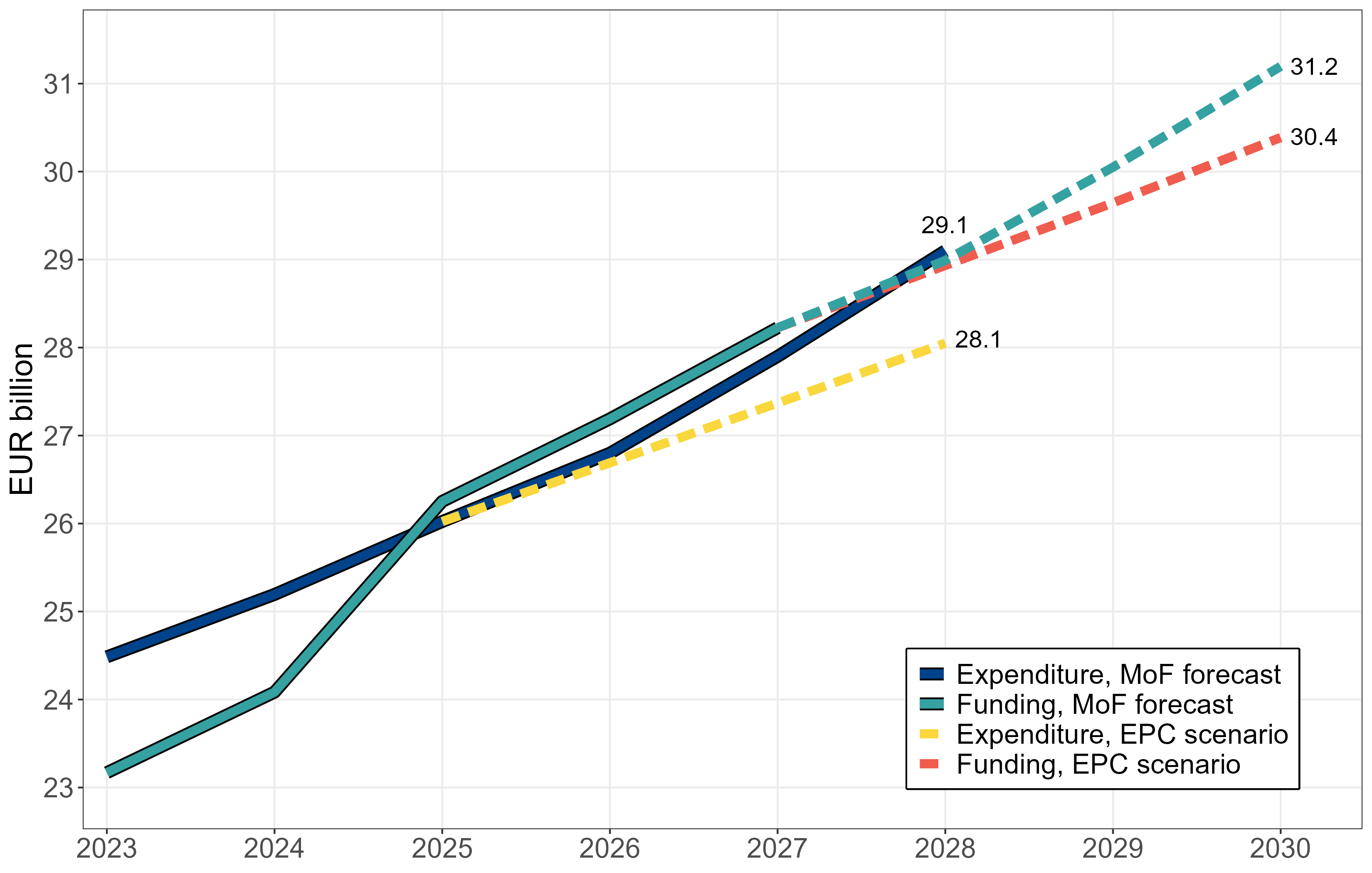
The blue line shows the combined realised expenditure of the WSCs in 2023–2024, expenditure based on the financial statement forecasts in 2025, and expenditure consistent with the Ministry of Finance forecast for 2026–2028. The solid green line shows central government funding for the WSCs in 2023–2027 based on realised expenditure, and the dashed green line shows central government funding for 2028–2030 if expenditure were to develop in line with the Ministry of Finance forecast. The dashed yellow line shows expenditure development based on the Council’s calculations, in which counties consolidate by a total of EUR 1 billion over 2026–2028, and the dashed red line shows the corresponding development of central government funding in 2028–2030 under this consolidation assumption. Source: Ministry of Finance, Council’s calculations.
Covering the EUR 2.2 billion accumulated deficit in WSC finances with corresponding surpluses by the end of 2028 would require average annual expenditure growth of 2.5 per cent over 2026–2028. This would mean that the annual growth in combined WSC expenditure would be approximately 1.5 percentage points lower than the 4 per cent annual growth in the Ministry of Finance forecast. In euro terms, this would correspond to spending cuts of approximately EUR 1 billion relative to the Ministry of Finance forecast in 2028.
Figure 3.2.2 also shows the development of central government funding resulting from such expenditure development. Lower expenditure growth would generate combined surpluses for the WSCs over 2026–2028. At the same time, it would keep central government funding after 2028 at a lower level than under the Ministry of Finance forecast expenditure path, as the ex-post adjustment that raises funding in line with realised expenditure would be smaller.
Below, we present a simplified calculation of how the approximately EUR 1 billion in expenditure consolidation relative to the Ministry of Finance forecast described above would be distributed across counties, if all counties were granted additional time to cover their deficits until the end of 2028.
Example of the consolidation requirement by county group
In Table 3.2.1, the wellbeing services counties are divided into four groups (I–IV) on the basis of their combined surplus or deficit accumulated over 2023–2025. Column (1) of the table shows the size of each county group measured by its share of total national funding in 2026. Column (2) shows the accumulated deficit in millions of euros over 2023–2025, and column (3) shows the accumulated deficit relative to 2026 funding.
|
| (1) | (2) | (3) | (4) | (5) | |
|
|
Share
of
WSC
finances,
% |
Accumulated
deficit,
EUR
m |
Accumulated
deficit,
% |
Avg.
max.
change
in
expend.,
% |
Total
consol.
by
2028,
EUR
m | |
|
| ||||||
|
| ||||||
| Counties I | 28 | 10 | 0 | 5.0 | +250 | |
| Counties II | 46 | -990 | -8 | 3.0 | -350 | |
| Counties III | 15 | -595 | -14 | 1.0 | -400 | |
| Counties IV | 10 | -625 | -22 | -2.0 | -500 | |
| WSCs total | 100 | -2200 | -8 | 2.5 | -1000 | |
Classification of counties: I: Counties that are likely to cover their deficits during 2026 (Länsi-Uusimaa and Pirkanmaa) and Helsinki. II: Counties with an accumulated deficit of 4–11% relative to 2026 funding (Kainuu, Kanta-Häme, Keski-Pohjanmaa, Pohjanmaa, Pohjois-Karjala, Pohjois-Pohjanmaa, Pohjois-Savo, Päijät-Häme, Satakunta, Vantaa ja Kerava and Varsinais-Suomi). III: Counties with an accumulated deficit of 13–17% relative to 2026 funding (Etelä-Karjala, Etelä-Pohjanmaa, Etelä-Savo, Keski-Uusimaa, Kymenlaakso). IV: Counties with an accumulated deficit exceeding 20% relative to 2026 funding (Itä-Uusimaa, Keski-Suomi and Lappi).
Accumulated deficit, EUR m (2) is calculated using 2023 and 2024 financial statement data and 2025 preliminary financial statement data. Accumulated deficit, % (3) is calculated by dividing (2) by each county’s 2026 funding. Total consolidation by 2028, EUR m in column (5) is calculated on the basis of the difference between the maximum change in expenditure in column (4) and the Ministry of Finance forecast, relative to the 2025 expenditure level of each county group.
Source: State Treasury, Ministry of Finance, Council’s calculations.
The starting assumption of the calculation is that county expenditure would grow at approximately 4 per cent annually in line with the Ministry of Finance forecast, if counties were to undertake no new consolidation measures. County-specific funding is assumed to develop in line with calculations published by the Ministry of Finance.9 In the illustrative calculation, the average annual change in expenditure over 2026–2028 that would allow each county group to just cover its accumulated deficit by the end of 2028 has been computed. This maximum annual average change in expenditure resulting from the obligation to cover deficits is shown in column (4) of the table.
The euro amount in column (5) represents the total required consolidation over 2026–2028 by county group. It is calculated as the difference between the maximum change in expenditure computed for each county group in column (4) and the Ministry of Finance forecast, relative to the combined 2025 expenditure level of each county group.
Column (5) of Table 3.2.1 shows how the combined consolidation of approximately EUR 1 billion at the national level would be distributed across county groups. It should be noted that there is still considerable county-specific variation in accumulated deficits and consolidation pressure within each group. Moreover, the results of the calculation are sensitive to assumptions about the timing of consolidation, as the assumption regarding 2026 consolidation affects 2028 funding through the ex-post adjustment. The illustrative calculation is intended only to provide a rough indication of the scale of consolidation that covering deficits by the end of 2028 would require from different counties.
Counties I: Helsinki has posted a slight surplus already in 2023–2025 (and would therefore already fall outside the scope of the proposed extension regulation). The calculation also assumes that Länsi-Uusimaa and Pirkanmaa will cover their deficits during 2026. The deficit-covering requirements would therefore not bind these three counties in 2027 and 2028. However, the calculation assumes that these three counties would aim to keep their finances in balance in 2027 and 2028.10 Under these assumptions, their expenditure could grow by an average of 5 per cent in 2026–2028, which would correspond to an expenditure increase of approximately EUR 250 million in 2028 relative to the Ministry of Finance forecast.
Counties II: For the 11 counties with accumulated deficits of 4 to 11 per cent relative to 2026 funding, expenditure could grow by an average of approximately 3 per cent per year over 2026–2028, approximately one percentage point less than in the Ministry of Finance forecast. In euro terms, this would correspond to consolidation of approximately EUR 350 million over three years relative to the Ministry of Finance forecast. These counties are most likely to be those that would meet the conditions for extending the deficit-covering period to either 2027 or 2028. The precise consolidation required of these counties thus also depends on the length of the extension granted. The consolidation requirement presented in the table for these counties can, however, be considered broadly realistic. These counties account for nearly half of the total WSC finances, so their expenditure development is of great significance for public finances as a whole.
Counties III: The five counties with accumulated deficits of 13 to 17 per cent relative to 2026 funding would need to keep their nominal annual expenditure growth at an average of 1 per cent over 2026–2028 in order to cover their deficits by the end of 2028. This expenditure growth rate would, for these counties, correspond to approximately EUR 400 million in lower expenditure in 2028 compared to the Ministry of Finance forecast. Some of these counties could meet the conditions for an extension of the deficit-covering period. However, covering deficits even by the end of 2028 may prove too demanding a target for some of these counties. The Government may therefore need to initiate assessment procedures also with some counties in this group.
Counties IV: The three counties in the weakest financial position would need to cut their expenditure in nominal terms by an average of just over 2 per cent annually over 2026–2028 in order to cover their deficits by the end of 2028. In euro terms, this would correspond to consolidation of EUR 500 million relative to the Ministry of Finance baseline forecast in 2028. In practice, however, these counties do not need to aim for such tight consolidation, as the government has already initiated assessment procedures with them. In simplified terms, the assessment procedure means that the fiscal consolidation of a WSC is determined in an assessment group established for the purpose. The consolidation timeline for these counties is thus assessed on a case-by-case basis.
The illustrative calculation presented above demonstrates how the scale of the required consolidation varies between counties in different financial positions, if all counties were to aim to cover their deficits by the end of 2028 at the latest. A few WSCs are likely to achieve a balanced financial position already during 2026, and these counties would even have room for expenditure increases. For the majority of counties, the additional time until the end of 2028 made available by the proposed legislative amendment should be sufficient to cover their deficits. However, it appears likely that for some counties, even the two-year extension will not be sufficient for achieving the necessary spending cuts.
The illustrative calculation uses financial statement forecast data for 2025. As noted above, the financial statement estimates reported in January 2026 indicate that the combined result of the WSCs would be better than the forecast data suggested. According to the estimate data, the 2025 result improved particularly for Helsinki, Vantaa-Kerava, Varsinais-Suomi and Länsi-Uusimaa. These counties in particular would have scope for larger expenditure increases than the maximum expenditure growth presented in Table 3.2.1. For the counties in the weakest financial position, the financial statement estimates do not indicate a significant change, meaning that the updated data would not materially alter the consolidation pressure presented in Table 3.2.1 for these counties. If the final 2025 financial statements confirm the developments indicated by the estimate data, the divergence between counties will be even more pronounced than presented here.
3.3 Needs-based allocation of funding
Central government funding for the wellbeing services counties is allocated on the basis of calculated factors. Approximately 80% of funding is allocated on the basis of county-specific health and social care service need. The calculation of service need is described in more detail in Text Box 3.1. Approximately 13% of funding is allocated on the basis of the county’s population. Other factors determining the allocation of funding include the share of foreign-language speakers, with a weight of approximately 2%, and the share of bilingual residents, with a weight of approximately 0.5%. In addition, county-specific transitional equalisation additions or deductions are applied to the county-specific imputed funding. These are calculated by comparing the combined 2022 expenditure of the municipalities in each county’s area with the county’s imputed funding at 2022 levels.
Development of the needs-based allocation of funding
The Finnish Institute for Health and Welfare (THL) calculates county-specific need coefficients annually on the basis of the most recent data on the use of services, such as diagnosis data collected by the counties and other morbidity data. Funding should thereby reflect changes in county-specific service need as accurately as possible. In counties where there has been an increase in (diagnosed/recorded) morbidity, funding rises to match the increased service need. However, the allocation of funding based on estimated service need is a zero-sum game between counties: funding correspondingly decreases in other counties if their morbidity levels have not changed.
In practice, however, diagnosis recording practices have varied across counties, and the data used by THL have also been affected by problems related to the transfer of diagnosis records and information systems. Some of the problems with the diagnosis data stem from the differing or deficient recording practices of municipalities, and the counties have sought to rectify these problems.11 As a consequence of problems related to diagnosis recording and data transmission, changes in county-specific need coefficients have not necessarily reflected changes in actual service need. Unforeseen changes in estimated service need and, consequently, in funding also complicate the counties’ financial planning. In addition, diagnosis-based funding creates a financial incentive to record certain types of diagnoses with a low threshold and, conversely, to economise on preventive services.
Problems associated with the assessment of service need could be significantly alleviated by discontinuing the use of morbidity data in the determination of county-specific service need. County-specific service need could be calculated more simply on the basis of population structure and certain socioeconomic factors.12 The advantage of such a model compared to the current one would be that the differing recording practices of counties and problems related to information systems would not affect the assessment of service need. As funding would no longer be based to a large extent on disease diagnoses, counties would have a clear incentive and opportunity to invest in disease prevention. Funding would also be more predictable than under the current model.
THL updates the need-factor model at least every four years, as required by law. In its most recent report on the update of the need-factor model (Holster et al., 2025), THL has calculated county-specific need coefficients using several alternative model specifications, one of which is based solely on population structure and certain socioeconomic factors. Although the addition of need factors slightly increases the models’ explanatory power at the individual level,13 a demographic model nevertheless produces, according to THL’s calculations, very similar results at the county level as the current model. In other words, although morbidity data naturally predict individual-level service need, their contribution to the assessment of county-level service need appears to be very limited. Given the potential ambiguities associated with diagnosis data, it is not clear that the current model produces even a marginally better estimate of actual service need across counties than a simpler model that disregards morbidity data.14
THL has, however, proposed an even more detailed and extensive use of morbidity data in the calculation of county-specific service need than is currently the case (Holster et al., 2025). This proposal could further exacerbate the problems described above with the current assessment of service need. In any case, different models should be evaluated solely on the basis of how well they capture service need across counties. The extent to which models predict individual-level service need should not be of relevance.
A transition from the current service need calculation, which includes a large number of disease categories, to a considerably simpler model would, of course, change the allocation of funding between counties to some extent. On the other hand, it should be noted that the more extensive disease classification proposed by THL would also change the allocation of funding relative to the status quo. The funding model should be assessed as a whole, including the shares of population-based allocation and other calculation factors as well as the basis for calculating transitional equalisations.
Text Box 3.1. Calculation of county-specific service need
The calculation of county-specific health and social care service need is based on research by the Finnish Institute for Health and Welfare (THL); see Häkkinen et al. (2020) and Holster et al. (2022). Service need is calculated for three service categories: healthcare, elderly care and social care.
For each of these service categories, a separate model has been constructed to predict the population’s service need, in which the costs of service use are modelled on the basis of need and supply factors. Service need is first predicted at the individual level and then aggregated into county-level need. Finally, county-level need is expressed relative to the national average, yielding county-specific need coefficients for healthcare, elderly care and social care, on the basis of which central government funding is allocated to the WSCs.
Healthcare and elderly care service needs are modelled statistically from individual-level register data covering the entire population. The healthcare service need calculation uses, as need factors, approximately 120 disease categories and socioeconomic factors in addition to population structure. The elderly care need factors include approximately 40 disease categories and socioeconomic factors in addition to the age groups of the elderly population. Social care need factors comprise approximately 30 disease categories and socioeconomic factors. However, the register data currently available for modelling social care service need are not as comprehensive as those used in the healthcare and elderly care models, which means that the social care calculation involves the greatest imprecision.
THL updates the need-factor model at least every four years. The diseases and socioeconomic factors describing service need under current legislation are set out in an annex to the Act on Funding for the Wellbeing Services Counties (617/2021). Although the need factors remain unchanged for four-year periods, the county-specific service need coefficients used in the allocation of funding are calculated annually on the basis of the most recent data on the use of services, such as diagnosis data collected by the counties. Funding should thereby reflect changes in county-specific health and social care service need as accurately as possible.
Update of the need-factor study in 2025 per the government programme
According to the government programme, the needs-based allocation of funding will be maintained but developed on the basis of research. THL has accordingly updated its need-factor model study, mainly by developing the disease classification and by taking supply factors into account more comprehensively than before. THL proposes increasing the number of disease categories so that the healthcare service need calculation would use approximately 190 disease categories. However, adding explanatory variables to the model does not materially increase the model’s explanatory power even at the individual level (see Holster et al. (2025), Tables 11–13).
3.4 Government targets for the wellbeing services counties
Central government funding for the wellbeing services counties is approximately EUR 27.2 billion in 2026, corresponding to 30 per cent of the central government budget appropriations for 2026. As a result of the statutory annual increases to funding, the level of funding is estimated to rise to approximately EUR 30 billion by 2029. WSC expenditure developments have a significant effect on the level of central government funding through the ex-post adjustment. Measures aimed at containing expenditure growth therefore have an impact on public finances as a whole.
Of the over EUR 9 billion in fiscal consolidation targeted by the government during the current electoral term, approximately EUR 1.8 billion is directed at WSC finances. Approximately half of this is intended to be achieved by reducing the statutory tasks and obligations of the WSCs and by cutting central government funding correspondingly, and approximately half through the counties’ own efficiency and savings measures.
The government is targeting a reduction in the statutory tasks of the WSCs totalling approximately EUR 900 million over the electoral term. The reduction of tasks and obligations is, in principle, neutral from the perspective of WSC finances, as central government funding is cut by an amount corresponding to the estimated reduction in expenditure at the national level resulting from the reduced tasks. From the perspective of central government finances, the reduction of statutory tasks strengthens the fiscal position in direct proportion to the funding cut. This, however, requires that funding is not cut excessively or too little relative to the actual savings. If funding is cut by more than the actual savings, the excess cut may leak back into national-level funding through the ex-post adjustment.
The government has largely implemented the reductions in tasks and obligations set out in the government programme as well as those decided in spring 2024. We described these measures in more detail in our previous annual report. It should be noted, however, that nearly half of the government’s savings decisions compensate for the higher-than-anticipated expenditure growth in 2023 and 2024 and the resulting ex-post adjustment to funding in 2025 and 2026.15 In addition, the implementation of some savings decisions has been delayed or the estimated savings effect has been revised, such that the impact of the appropriation cuts is currently estimated to fall approximately EUR 200–300 million short of the government’s target.16
It is, however, positive that the government has taken measures to ensure that the rapid expenditure growth of the WSCs in their early years does not translate fully into increased central government sector borrowing. Although the measures do not directly strengthen WSC finances, they may have an indirect effect, for example through improved availability of personnel. This may already be reflected in the reduced use of agency staff by the WSCs.
In addition to the measures that directly reduce central government funding, the government targets a strengthening of public finances through the counties’ own productivity and savings measures of EUR 900 million by 2027. The WSCs should thus achieve permanent savings of just under EUR 300 million per year in 2025–2027.
If realised, the counties’ own efficiency measures would strengthen WSC finances immediately, and central government finances with a two-year lag through a lower ex-post adjustment. The target is, in itself, commendable, as moderate expenditure development also keeps the growth of central government funding moderate. However, assessing the attainment of the target is inherently difficult, and the divergence in county finances complicates this further. In the current model, the pressure on counties to improve their efficiency stems fundamentally from the binding nature of the deficit-covering period, not from the target set out in the government programme. Moreover, it is possible that counties improve their operations as targeted but that the benefits are not realised as a strengthening of public finances, but rather as improvements in the level of services. The counties are likely to pursue such improvements even without government direction.
3.5 On the incentives in the funding model
At present, the most significant incentive or pressure to contain expenditure growth stems from the binding nature of the deficit-covering period. Due to the substantial accumulated deficits, the consolidation pressure will continue in the near term for all counties that do not manage to cover their deficits by the end of 2026. These counties account for approximately 70% of total WSC finances but differ considerably from one another.
As described above, approximately half of the WSCs are likely to receive additional time to cover their deficits as a result of the proposed regulatory change, in which case they would face pressure for significant expenditure discipline also in 2027 and 2028. The greatest consolidation pressure falls on those counties with the largest accumulated deficits. For these counties, however, the consolidation pressure arising from the obligation to cover deficits is spread over a longer period, as agreed in the assessment procedure between each county and the government.
For the few counties that the obligation to cover deficits is unlikely to bind after the end of 2026, the current model does not necessarily provide strong incentives to contain expenditure growth. These counties would in fact have scope for expenditure increases. The three strongest counties already account for close to 30 per cent of WSC finances, meaning that their expenditure development has a significant effect on expenditure development at the national level and on the resulting ex-post adjustment. From the perspective of public finances, it would therefore be important to assess how the incentives for these counties to contain expenditure growth could be strengthened.
One way to improve the incentives in the funding model would be to grant the counties the right to levy taxes. Regional taxation could improve the counties’ incentives to improve their operational efficiency by giving the WSCs the possibility to lower the tax burden on their residents as a result of savings. In the current model, it is always in the counties’ interest to spend all of the funding allocated to them.
The Economic Policy Council described the various perspectives related to regional taxation more comprehensively in connection with the county reform prepared during Prime Minister Sipilä’s government term.17 (EPC (2019); see also Haveri et al. (2025), pp. 75–78). The committee on regional taxation, which operated during Prime Minister Marin’s government term, concluded that the right of the WSCs to levy taxes should be examined once sufficient experience has been gained regarding the functioning of the WSC funding model (Finnish Government, 2021). However, the government programme of Prime Minister Orpo states that the government will not introduce WSC taxation and will not prepare any studies related to it during this electoral term.
One argument put forward in favour of regional taxation is that it would provide better incentives for containing expenditure growth than full central government funding. Central government funding is associated with the so-called soft budget constraint problem, as counties have no incentive to operate efficiently if they know that the central government will be compelled to grant them additional funding to safeguard services.
The soft budget constraint problem has not, however, materialised to any significant extent so far: in 2025, six counties applied to the central government for additional funding totalling approximately EUR 430 million. The government, however, decided to grant additional funding to only one county, Pohjois-Karjala, in the amount of EUR 2.6 million. The government’s decision to grant additional time for covering deficits also partly mitigates the soft budget constraint problem, as it gives counties a better opportunity to balance their finances without compromising essential services. Spreading the consolidation over several years does not necessarily mean an increase in total expenditure in the near term.
3.6 Council views
Although the financial situation of the wellbeing services counties has improved considerably and turned to surplus in 2025, the counties still have approximately EUR 2 billion in uncovered accumulated deficit at the end of 2025. The difficult financial situation is largely attributable to the rapid expenditure growth in 2023 and the fact that funding was adjusted to match realised expenditure only in 2025. For several counties, it is impossible to cover their accumulated deficit solely through expenditure consolidation.
It is positive that the government has responded to the financial situation of the WSCs by extending the deficit-covering period. This gives many counties a much more realistic opportunity to balance their finances without compromising essential services. Regrettably, however, the financial situation of the counties has diverged significantly. For some counties, even a two-year extension of the deadline is unlikely to be sufficient. More counties may therefore still become subject to the assessment procedure.
The binding nature of the deficit-covering period compels the majority of counties to achieve spending cuts in order to contain expenditure growth also in the coming years. There are, however, a few counties that do not have a strong incentive to implement spending cuts, for example by scaling back services whose benefits are considered small relative to their costs. By default, it is in the counties’ interest to spend all of the funding they receive. The development of the funding model should therefore focus in particular on how the incentives for these counties can be strengthened.
One possibility would be to grant the counties the right to levy taxes. This would give the WSCs the opportunity to lower the tax burden on their residents as a result of savings. It would also increase the predictability of WSC funding compared to the current model.
The right to levy taxes does, however, pose certain problems. For example, the WSCs would not have a strong incentive to take into account how their taxation affects the rest of the public sector. Counties also differ in their capacity to collect tax revenues. If the right to levy taxes were introduced, it would therefore probably be advisable to add, in addition to the need-based component, a tax revenue equalisation element to central government funding, similar to the arrangement that exists in central government funding of municipalities.
Central government funding of the wellbeing services counties should ideally reflect regional service need as accurately as possible. The calculation of county-specific service need is based to a large extent on morbidity data derived from various healthcare diagnosis records. However, diagnosis recording practices have varied across counties. This has undermined the alignment of funding with actual service need and has created difficult uncertainty for the WSCs regarding their future funding. Diagnosis-based funding also creates a financial incentive to record certain types of diagnoses with a low threshold and, conversely, to economise on preventive services.
These problems could be significantly alleviated by discontinuing the use of morbidity data in the allocation of funding between counties. Although morbidity data are a good predictor of individual-level service need, calculations by THL suggest that their contribution to the assessment of county-level service need is very limited. In other words, county-level service need can apparently be estimated almost as well — or as poorly — on the basis of demographic and socioeconomic factors alone that do not depend on the counties’ own recording practices or diagnoses. It is not entirely clear why the assessment of service need has relied on detailed morbidity data.
4 The Finnish public sector balance sheet
Finland’s general government has both debt and assets. The vast majority of its financial assets consists of investment assets in the earnings-related pension system. Their purpose is to cover a portion of future earnings-related pension expenditure. Financial liabilities, such as the debt taken on by central and local government, and financial assets can be aggregated into net financial assets. On the other hand, accrued earnings-related pension entitlements can, in an even broader examination of the public sector balance sheet, be counted among the liabilities of the public sector.
In this chapter, we first introduce the concepts relating to public sector net wealth and examine the developments in the main items of the Finnish public sector balance sheet in the 2000s. The analysis draws extensively on the background report written for the Economic Policy Council by Juha-Matti Tauriainen (Tauriainen, 2026). We then discuss the pension reform, interest-subsidy loans associated with publicly subsidised housing production and government guarantees, as well as the additional withdrawal from the State Pension Fund to the central government budget decided by the government at its spring 2025 spending limits session. All of these have a direct impact on the public sector balance sheet.
4.1 Balance sheet items and net wealth of the public sector
The assessment of public sector fiscal sustainability has traditionally been based on the gross debt and general government deficit relative to GDP, in accordance with the criteria set out in the European Union’s Maastricht Treaty. According to one definition, public sector debt is considered unsustainable if “it cannot be repaid without altering the contractual terms of the debt or rendering them irrelevant, via default, restructuring, or hyperinflation” (Willems and Zettelmeyer, 2022).
On this basis, it is important to distinguish between debt sustainability and fiscal sustainability. Fiscal policy is unsustainable if debt cannot be stabilised or reduced through current fiscal policy measures. In such a situation, investors’ willingness to refinance government debt may also weaken as the budget deficit grows, which in turn raises the refinancing rate on public debt. By contrast, the level of debt or the debt ratio is unsustainable only if the debt cannot be repaid under any conceivable fiscal policy arrangement. For this reason, the assertion that debt or the debt ratio is at an unsustainable level is considerably stronger than the assertion that fiscal policy is on an unsustainable path (Darvas et al., 2025).
However, gross debt and the deficit provide only a partial picture of the state of public finances. Gross debt describes the total amount of general government liabilities but does not take into account the assets available to cover those liabilities. Moreover, measuring gross debt at nominal value does not account for changes in market values, interest rate developments, or the maturity structure of bonds. This may lead to situations in which the financial risks of the public sector are assessed inadequately, particularly in the context of macroeconomic shocks or large investment needs. A focus on gross debt may also encourage creative accounting, whereby the debt measure is artificially improved without genuinely strengthening the fiscal position (Koen and Van den Noord (2005); Milesi-Ferretti (2004); von Hagen and Wolff (2006)).
Recent research and international organisations such as the OECD and the IMF have stressed the importance of public sector net wealth in assessing fiscal sustainability, alongside these indicators (Chai et al. (2024); Hadzi-Vaskov and Ricci (2022); Minarik (2024)). Net wealth provides a broader perspective on the financial position of the public sector.
The scope of net wealth
Net wealth measures the difference between general government assets and liabilities. In addition to financial assets, it covers in principle also non-financial assets, such as infrastructure and buildings, as well as future pension obligations promised on the basis of previous earnings and falling under public sector responsibility, such as accrued earnings-related pensions in Finland. The aim of this measure is to provide a comprehensive account of both assets and liabilities and to reveal hidden liabilities that are passed on to future generations.
Examining net wealth can alter the interpretation of fiscal sustainability, particularly in situations where assets grow faster than liabilities or where pension liabilities constitute a significant share of future obligations. Net wealth also provides a means of identifying accounting embellishment, as it is not confined to debt alone but takes the broader public sector balance sheet into account. This broader perspective can be particularly important when assessing the capacity of the public sector to manage economic challenges and maintain the confidence of financial markets.
Many advanced economies, including the Nordic countries, the United Kingdom, Australia, New Zealand, and Canada, have developed their public sector accounting systems so that the various components of the balance sheet can be constructed. International Financial Reporting Standards (IFRS) define assets and liabilities as rights and obligations based on contracts, legislation, and past events that have economic value. However, the preparation of public sector balance sheets does not follow fully harmonised international standards, which means that the coverage and comparability of balance sheets vary across countries. Estimating the magnitude of some public sector liabilities is also difficult. This applies, for example, to many government guarantees.
Indicator developments
In the calculations presented by Tauriainen in accordance with the European System of National and Regional Accounts (ESA 2010), the main components of Finnish general government net wealth in 2024 were the financial assets of general government (EUR 414 billion), financial liabilities (EUR 254 billion), non-financial assets (EUR 217 billion), and earnings-related pension liabilities (EUR 945 billion). A more detailed description of the net wealth components can be found in the background report (Tauriainen, 2026).
Examining the development of Finnish general government net wealth reveals that global economic crises, such as the financial crisis of 2007–2008 and the COVID-19 pandemic in 2020, have had a significant impact on both debt and asset levels (see Figure 4.1.1 and Tauriainen (2026)). The trends in net wealth and net financial assets reflect both changes in financial markets and developments in the real economy. Growth in gross debt during times of crisis does not, therefore, alone describe the true financial position of the public sector; examining net wealth reveals how assets and liabilities evolve in relation to each other.
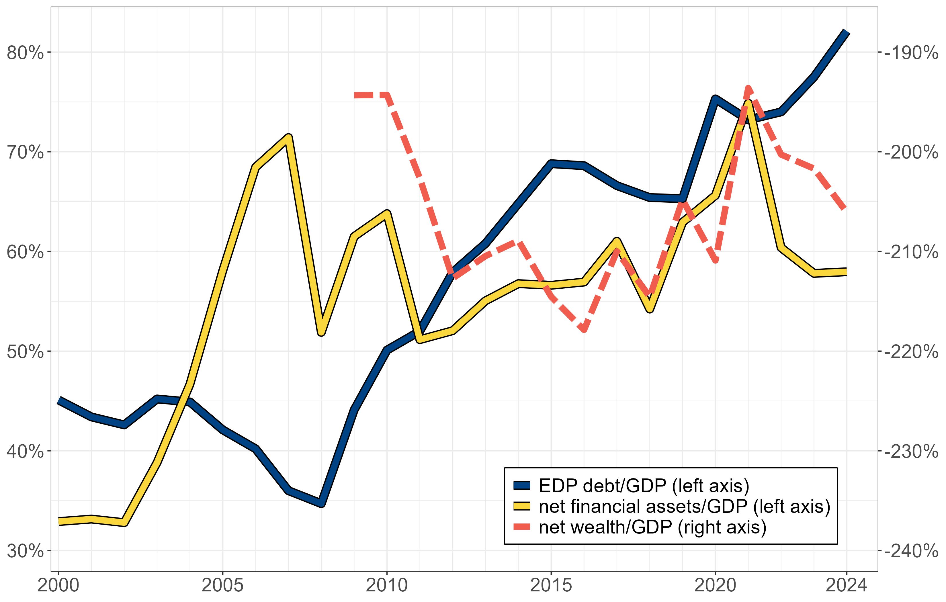
Source: Tauriainen (2026).
Pension liabilities are estimated by calculating the present value of accrued pensions, that is, by discounting future pension payments to the present day. The valuation of non-financial assets, such as infrastructure, is based on fair value, which reflects maintenance costs and market-based value rather than merely an accounting entry.
Economic policy measures, such as infrastructure investments, the sale of equity holdings, and the use of pension funds, affect different parts of the general government balance sheet. For example, financing infrastructure investments by selling equity holdings reduces financial assets but does not change net wealth at all.
On the basis of Figure 4.1.1, it is clear that the development of the public sector gross debt ratio and net wealth diverge from time to time, providing a different picture of the state of public finances. For instance, the net wealth-to-GDP ratio has not exhibited the same deteriorating (downward in the figure) trend from 2008 onwards as the debt ratio. Recent developments are, however, concerning from the perspective of both indicators. Gross debt has grown relative to GDP, and net wealth, which is dominated by pension liabilities, has become increasingly negative relative to GDP. Net financial assets, by contrast, have remained relatively stable relative to GDP since 2022. This has been supported by the increase in the value of financial assets and the decline in the market value of public debt as a result of rising interest rates.
4.2 Pension reform
The government set out in its programme the objective of a pension reform that would strengthen public finances and stabilise the development of the earnings-related pension contribution through a rules-based stabilisation mechanism. The government published a draft proposal for the pension reform in December 2025.18
The most important element of the reform concerns the investment activities of private earnings-related pension providers. The reform directs these providers, such as Ilmarinen and Varma, to invest a larger share of earnings-related pension assets in equities and other relatively high-risk investment instruments. The objective is to achieve higher average returns for the pension funds. Among public pension providers, at least Keva’s investments have historically performed better owing to a higher-risk investment strategy.
Under the reform, the private-sector earnings-related pension contribution is fixed at 24.4 per cent for 2026–2030. In addition, the pre-funding of old-age pensions is slightly increased, so that a larger share of earnings-related pension contributions is directed towards saving for future pensions. This represents responsible policy from the perspective of the long-term sustainability of the earnings-related pension system: the expected increase in investment returns resulting from greater risk-taking is not immediately extracted through a reduction in the pension contribution. On the other hand, the reform does not immediately create room to raise other taxes without increasing the overall tax burden.
Pension benefits are affected by the reform only through the so-called index limiter. This reduces pension index increases in situations where inflation exceeds the growth of nominal wages for at least two years. Historically, situations in which this mechanism would have had a significant effect on pensions have been relatively rare.
Impact of the reform on public finances
According to an estimate calculated at the Ministry of Finance, the reform strengthens public finances, as measured by the change in the sustainability gap, by 0.8 percentage points relative to GDP. The estimate is based on an analysis examining a large number of stochastic paths or scenarios produced by the Finnish Centre for Pensions, in which the investment returns of earnings-related pension assets evolve in different ways.19 The sustainability gap is first calculated separately for each path with and without the reform. Higher investment returns imply a lower earnings-related pension contribution at some point in the future. This narrows the sustainability gap by reducing the increase in the overall tax burden required to balance public finances as a whole. The calculations do not seek to capture possible general equilibrium effects, for example through the response of wages.
The pension reform affects the development of public finances differently across different paths. The reform leads to a higher earnings-related pension contribution and a correspondingly larger sustainability gap on paths where the higher investment risk frequently materialises as poor investment returns. The Ministry of Finance’s estimate of the reform’s impact on the sustainability gap is, strictly speaking, the median of the effects calculated across the different paths. In other words, public finances strengthen by more than this in half of the paths examined and by less in the other half. The positive median effect primarily reflects the higher investment risk and increased pre-funding.20 The impact of the index limiter is smaller than these.
It should be noted that although a decline in the earnings-related pension contribution expands certain tax bases, it fully strengthens public finances in line with the calculations only if it is accompanied by a corresponding tightening of other taxation.
A calculation based on the mean would yield a more favourable estimate of the reform’s impact on the sustainability gap. This is because, on some paths, very high investment returns lead to very large investment assets, enabling the earnings-related pension contribution to be reduced to very low levels, whereas the impact of poor investment returns is bounded by the fact that earnings-related pension assets cannot become negative.
On the other hand, the risks are also highly asymmetric from the perspective of welfare: we would presumably wish to avoid a situation in which earnings-related pension assets shrink to very low levels, even if the price were to forgo the possibility of achieving a very low pension contribution. Financial difficulties in the earnings-related pension system may also coincide with other factors that weaken public finances, making the overall situation more difficult to manage.
Emphasising the median effect rather than the mean effect can be seen as one way of accounting for the costs of increased risk. However, increasing investment risk would strengthen fiscal sustainability even as measured by the median effect, even if investment risk were initially at a much higher level than at present. This certainly does not mean that investment risk should be increased without limit. The merits of increasing the investment risk of earnings-related pension providers cannot, therefore, be assessed without taking a position on how risks are viewed or how well they can be managed. This is acknowledged in the government’s draft proposal for the pension reform. By contrast, in public debate, the effect of the pension reform in strengthening public finances has frequently been cited without any mention of the associated risks.
A situation in which pensions grow faster than wages creates upward pressure on pension contributions. The index limiter included in the reform therefore probably somewhat stabilises the earnings-related pension contribution. It does not, however, directly link pensions to the long-term financial balance of the system, which is also affected by investment returns.21
The fact that the reform does not introduce a rules-based stabiliser more significant than the index limiter leaves it unclear how benefits and contributions would be adjusted if investment returns develop very differently from current expectations. This is ultimately a question of how economic risks are to be shared among, for example, employees and retirees or members of different generations. The current system rests on the premise that, ultimately, the earnings-related pension contribution adjusts. This leaves the investment risks largely on the shoulders of employees. A significant increase in the pension contribution may not even be a credible option, as it would have adverse repercussions for the rest of public finances.
Key elements of the reform regarding pension providers’ investment activities
One of the most significant changes concerning the investment of earnings-related pension assets is the raising of the upper limit for the equity share of private pension providers from 65 per cent to 85 per cent relative to total investments. At the same time, the upper limit of the equity-linked buffer is raised from 20 per cent to 30 per cent. This allows pension providers a larger equity buffer against market fluctuations, as the equity-linked buffer responds to equity market developments in such a way that a provider’s solvency is not immediately jeopardised by poor returns. The increase in the buffer functions as a flexibility mechanism that smooths the significance of equity return fluctuations relative to the market situation and affects the extent to which a pension provider can recognise investment returns in its profit. When the upper limit of the equity-linked buffer is reached, the excess is recognised in profit.
The prudential level of the solvency limit is slightly reduced, enabling riskier investments and reducing pressure for forced sales during unfavourable market conditions. Investment losses weaken solvency, but with a lower prudential level, short-term equity price fluctuations do not cause a breach of the solvency limit as easily as before. The reduction in the prudential level therefore allows pension providers to make riskier investments. If the limit is nevertheless breached, the pension provider cannot, for example, pay client rebates.
The increase in the equity share is justified primarily by the long-term return expectations of equity markets. International equity markets have developed positively in the long term since the financial crisis, but a higher equity share also exposes investments to market risks and value fluctuations, as was seen during the COVID-19 crisis.
The Finnish Centre for Pensions estimates that the investment reform will increase the real returns of private pension providers by 0.2–0.4 percentage points over the long term. This improves the funding base of the pension system and may enable a reduction in the earnings-related pension contribution. On the other hand, the risk profile increases, which adds to the volatility of pension asset values at least in the short term.
From the perspective of joint liability, the collective nature of the equity-linked buffer distributes risk more broadly across the entire pension system, as it enables an individual provider to increase its equity risk without its solvency risk increasing. Since each individual provider recognises this opportunity, it becomes all the more important for the risk management of the pension system as a whole that all providers engage in active risk management and diversify their investments internationally.
From the perspective of system-wide risk management, it would also be important that the reform does not lead to pension providers’ investment strategies becoming even more similar. In addition, the integrating ESG (Environmental, Social & Governance) considerations into investment activities becomes all the more important if the share of international investments grows.
Pension benefits as part of the social security system
According to the government programme, the government aims for a significant strengthening of public finances without raising the overall tax burden while avoiding cuts that particularly weaken the position of the most vulnerable. With this objective in mind, it is useful to divide pension benefits roughly into three groups according to how their financing tightens the taxation of labour and how clearly they are targeted at low-income individuals.
One group consists of benefits that are precisely targeted at low-income individuals and whose financing clearly tightens the taxation of labour. These benefits include in particular the national pension and the guarantee pension. They are paid only to individuals whose career earnings and the resulting earnings-related pension remain relatively low. They weaken work incentives, as they are largely financed through taxes on labour and, in addition, higher earnings reduce the benefits at the individual level. The guarantee pension in particular has a negative effect on the work incentives of individuals who are low-income as measured by lifetime earnings. If an individual’s earnings-related pension is in any case going to remain below approximately EUR 1,000 per month, increasing the pension accrual, for example by extending the working career, does not increase their future pension at all, since the earnings-related pension reduces the guarantee pension on a one-for-one basis.
The second group consists of benefits that are not specifically targeted at low-income individuals but whose financing does not, on the other hand, tighten taxation or the tax wedge on labour at least to the full extent. This group includes earnings-related pensions accrued on the basis of earnings from work, which are financed by the earnings-related pension contribution. Higher earnings accrue a larger benefit, so this is not an income transfer specifically targeted at low-income individuals. The portion of the earnings-related pension contribution levied to finance such earnings-related benefits can, on the other hand, be regarded at least partly as a compulsory insurance premium rather than a tax on labour. This is because there is a clear link between the contribution and the benefit at the individual level: higher contributions generally result in a larger benefit. (As already described above, this does not, however, apply to individuals who receive the guarantee pension.) Therefore, these benefits and the contributions collected to finance them do not together tighten the taxation of labour to anything close to the full extent.
The third group comprises benefits that are not clearly targeted at low-income individuals but that nevertheless require tighter taxation. Such benefits include at least the pension accruing from academic degrees, the pension accruing from earnings-related unemployment periods, the survivor’s pension, and the pension accruing from periods of parental allowance.
Pensions accruing from academic degrees tend to benefit higher-income individuals, as a higher education degree leads to greater pension accrual than a vocational qualification, and the average lifetime earnings of graduates are higher than those of individuals with less education.22 The pension accruing from earnings-related unemployment periods is likely to be better targeted at low-income individuals as measured by lifetime earnings, since they are more frequently unemployed than others. However, the targeting is not very precise either: for example, higher-paid individuals receive higher unemployment compensation and therefore accrue more pension from unemployment than lower-paid individuals. Both students and unemployed persons are also presumably better served by financial support during the period of study or unemployment, when they have little other income, than by additional pension income received possibly only decades later.
The survivor’s pension is larger the smaller the surviving spouse’s own accrued earnings-related pension. Its recipients are therefore generally relatively low-income. On the other hand, it is larger the higher the earnings-related pension of the deceased spouse. It is thus not specifically targeted at low-income couples but rather benefits couples in which the spouses have very different levels of income. Pensions accruing from periods of parental allowance are essentially an income transfer to individuals with children, which is presumably the intention.
The pension benefits in this third group are financed through taxes and contributions that do not involve the same link between the contribution and the benefit as benefits accruing from work. For example, pensions accruing from academic degrees and from periods of parental leave are financed directly from the central government budget, while pensions accruing from unemployment periods are financed by the unemployment insurance contribution. Nor do couples who may benefit from the survivor’s pension pay a higher earnings-related pension contribution or any other charge than other individuals. Financing these benefits therefore requires higher taxation.
Cutting in particular some of the benefits belonging to the third group described above would appear to be a natural way to strengthen public finances within the constraints the government has set for itself. Against this background, it can be regarded as inconsistent that the pension reform does not seek greater savings through benefit cuts, especially given that the government has already cut certain income transfers, such as the general housing allowance, which can be considered more important for economically vulnerable individuals than some of the pension benefits mentioned above. Thanks to the guarantee pension, cuts to these pension benefits would not affect those receiving the smallest pensions at all.
The potential for savings from pension benefits generally depends critically on whether already accrued pensions are fully protected from cuts or not. Fully protecting already accrued pension entitlements often substantially reduces the potential for savings. Cutting already accrued pension entitlements is, of course, in principle more problematic than cutting future pension accruals. On the other hand, the longer pension entitlements are allowed to accrue, the greater the cost that their financing ultimately imposes on public finances.
The benefits belonging to the third group described above naturally account for only a small share of total pension expenditure. The sums involved are nevertheless not negligible when compared, for example, to the social security cuts already implemented by the current government. Ilmakunnas et al. (2024), for instance, estimate that pensions paid on the basis of academic degrees will rise to approximately two per cent of total earnings-related pension expenditure by 2080, which corresponds to approximately EUR 700 million per year relative to earnings-related pension expenditure in 2024. Under the current system, this will be reflected as a corresponding expenditure item in the central government budget. For now, the amount is much smaller, as pensions began to accrue from academic degrees only with the 2005 pension reform.
Pensions accruing from earnings-related unemployment periods are financed through unemployment insurance contributions, whereby the Employment Fund pays the earnings-related pension system a contribution corresponding to the pension accrual from unemployment periods. In recent years, this has resulted in an annual expenditure of approximately EUR 700 million for the Employment Fund. Family pension expenditure, which is mainly financed by earnings-related pension contributions, was approximately EUR 2 billion in 2024, the majority of which consisted of survivor’s pensions. In 2022, survivor’s pensions were made fixed-term, which limits survivors’ pension expenditure in the future. At the same time, however, eligibility for the survivor’s pension was extended to cover cohabiting partners as well.
4.3 Liabilities associated with publicly subsidised housing production
The government has decided to dissolve the National Housing Fund and to transfer its assets and functions to the central government budget from the beginning of 2026. This will increase budgetary revenue on a one-off basis by approximately EUR 2 billion as a result of the transfer of the fund’s cash holdings, even though the fund was already part of central government before its dissolution. The dissolution does not change the total wealth of the public sector (Tauriainen, 2026).
The transfer releases the housing fund’s assets for general use by central government. On the other hand, expenditure previously paid from the fund, such as interest subsidies related to interest-subsidy loans granted to ARA rental dwellings and right-of-occupancy housing, as well as various investment grants for construction, will henceforth appear in the central government budget.
The aforementioned interest-subsidy loans have been included in EDP debt since June 2022. According to calculations by Statistics Finland, the new method of calculation results in a debt ratio 5.9 percentage points higher than under the old method of calculation as measured in 2021.
Interest-subsidy loans give rise to interest rate risk and guarantee liability risk for the state. Interest rate risk materialises when the rate on an interest-subsidy loan exceeds the threshold, generating interest subsidy expenditure for the state. In June 2023, the National Housing Fund had a guarantee stock of EUR 17.4 billion from corporate loans (rental and right-of-occupancy guarantees) (Lahtinen et al., 2024). These corporate loan guarantees constitute contingent liabilities that cover approximately 25 per cent of the state’s total guarantee and warranty liabilities of approximately EUR 68 billion. According to the State Treasury, interest subsidy expenditure on interest-subsidy loans amounted to EUR 230 million in 2024 and EUR 130 million in 2025. The assets of the fund transferred to the central government budget may not even be sufficient to cover the liabilities related to interest subsidies alone (Lahtinen et al., 2024).
The National Audit Office assessed in its 2023 performance audit of the Housing Finance and Development Centre (ARA) that the probability of guarantee liability risk materialising was low (National Audit Office, 2023). The materialisation of guarantee liabilities would require significant underutilisation of dwellings, resulting in housing companies or right-of-occupancy associations losing rental income or maintenance charge revenues. The risk of underutilisation is greatest in areas where the quality-adjusted market rent is close to or even lower than the rent or maintenance charge based on the cost-recovery principle. Rental housing companies and right-of-occupancy associations can reduce the risk arising from the underutilisation of individual properties through regional equalisation of rents and maintenance charges, but if their properties are mainly located in a single municipality, this risk diversification may not be very effective.
There is reason to believe that the probability of guarantee liability risk materialising has grown in recent years. The rise in interest rates and other costs that began in 2022 has significantly increased maintenance charges and rents based on the cost-recovery principle. If maintenance charges rise close to the market rents of comparable dwellings, right-of-occupancy residents have an incentive to redeem their right-of-occupancy payment and move to a rental or owner-occupied dwelling. In such a situation, it is difficult for the association to find a new right-of-occupancy resident. It is likewise easy for a resident of a subsidised rental dwelling to move to a market-rate rental dwelling in a housing market situation where cost-recovery rents approach or even exceed the market rent level in the area. In these situations, the subsidised housing stock becomes underutilised and the rental and maintenance charge revenues of the companies decline, raising the risk of guarantee liabilities materialising.
From 2026 onwards, the state will not grant guarantees or interest subsidies for new right-of-occupancy dwellings. This may lead to an increase in maintenance charges in the existing stock. This is due to the back-loaded amortisation structure of interest-subsidy loans, which means that the debt servicing costs of new properties are low in the early stages of the loan and rise over time. The low debt servicing costs of new properties have been used to equalise maintenance charges across the entire housing stock of the same operator. In the future, this possibility will no longer exist.
Despite the increased risks described above, it is clear that interest-subsidy loans are not directly comparable to government bonds as public sector liabilities. In expected value terms, only a relatively small share of them will ultimately constitute a burden on taxpayers.
4.4 Additional withdrawal from the State Pension Fund
The government decided at its spring 2025 spending limits session on a one-off additional withdrawal of approximately EUR 1 billion from the State Pension Fund to the central government budget in 2027. The decision reduces the central government deficit and overall public sector borrowing by the same amount in 2027. However, the additional withdrawal does not affect the general government deficit as a whole, nor does it change the net financial assets of the public sector: financial assets decrease (as the investment assets of the State Pension Fund are reduced) by the same amount as financial liabilities compared to the situation without the additional withdrawal.
The additional withdrawal has been criticised on the grounds that the return on the State Pension Fund’s investments is likely to be higher than the interest rate on government debt. In that case, the total investment returns of the public sector would decrease by more than the amount the state saves in interest expenditure through lower borrowing. This is not, however, a conclusive argument against the additional withdrawal, since by the same logic the state should borrow additional funds without limit and invest the proceeds in, for example, equity markets. Such a strategy would, however, increase the risks to public finances without limit by raising debt relative to investment assets, the value of which can fluctuate.
The additional withdrawal of EUR 1 billion in question does not, of course, have a particularly large impact on public finances. In assessing it, however, it would be appropriate to also emphasise the management of risks to public finances, rather than focusing solely on expected return differentials or the near-term development of gross debt. The same perspective applies, for example, to the potential sale of government equity holdings.
4.5 Council views
In assessing public finances, it is important to examine not only liabilities but also the assets of general government. Net wealth aims to comprehensively account for financial assets and financial liabilities, pension liabilities, and the value of non-financial assets. Measuring it does, on the other hand, require various assumptions and demarcations that complicate at least international comparisons.
The fact that Finnish public finances hold substantial financial assets is likely to support Finland’s sovereign creditworthiness in the eyes of investors and thereby moderate the servicing costs of public debt. This does not, however, eliminate the need to contain the growth of the debt ratio. Increasing indebtedness raises risks to public finances even when it is matched by financial assets, since the value of financial assets can fluctuate significantly. It should also be noted that, in the broader examination of the public sector balance sheet, the earnings-related pension funds within the public sector are matched by large pension liabilities.
The pension reform proposed by the government is primarily an investment reform. The objective is to raise the returns of pension funds by increasing their equity share. The reform is likely to strengthen public finances by enabling a reduction in the earnings-related pension contribution in the future compared to the situation without the reform. This is based above all on increasing the investment risk of the pension funds. It is therefore regrettable that the reform did not include an agreement on a rules-based stabiliser that would define more credibly than the current arrangements how increased investment risks are shared among, for example, employees, retirees, and members of different generations.
The reform reduces pension benefits only in situations that, based on prior experience, are assessed to be relatively rare, namely those in which inflation exceeds the growth rate of wages for an extended period. Given the challenges facing public finances, the government’s related objectives, and the fact that other social security benefits have already been cut, it would have been consistent to also direct more significant cuts at future pension benefits in the reform.
In light of the government’s stated objectives, it would be warranted to re-examine in particular those benefits that are not accrued through work but that are also not clearly targeted at low-income individuals. Examples of such benefits include pensions accruing from academic degrees and from earnings-related unemployment periods, as well as the survivor’s pension.
Eliminating the pension accrual from earnings-related unemployment periods and the survivor’s pension would allow an immediate reduction in the earnings-related pension contribution or the unemployment insurance contribution, even if already accrued benefits were left entirely untouched. The trajectory of contributions would, of course, depend on how the resulting decrease in future benefit expenditure is factored into the calibration and timing of contributions and their pre-funding.
An immediate reduction in social insurance contributions would create room for an immediate tightening of other taxation without an increase in the overall tax burden. Unlike the proposed pension reform, such a package of measures would help reduce public sector indebtedness already in the near term. It would not, on the other hand, immediately reduce people’s disposable income. This would support aggregate demand in the near term compared to many of the social security cuts already implemented.
The additional withdrawal of EUR 1 billion from the State Pension Fund to the central government budget decided by the government in spring 2025 is an example of a measure that reduces the debt ratio but does not improve the sustainability of public finances, at least not in expected value terms. This is well illustrated by the broader examination of the public sector balance sheet, as the measure does not directly affect public sector net wealth.
The additional withdrawal can in principle be regarded as a reasonable measure. It somewhat reduces future investment returns but also the risks associated with the development of net wealth. Such measures should, however, rest on a predictable and clearly defined plan for managing the public sector balance sheet. Unpredictable additional withdrawals of this kind do not, for example, facilitate the investment activities of the State Pension Fund.
The government has indicated that it will reform the self-employed persons’ pension system so that the pension contribution of the self-employed is determined more clearly on the basis of their actual income than at present. Entrepreneurs’ organisations, for their part, have demanded that the self-employed should be allowed to determine their pension contribution more freely. Broad freedom of choice is, however, a problematic starting point from the perspective of the social security system as a whole. It would, for example, make it possible to increase the amount of the national pension by minimising the earnings-related pension accrual — and the associated contribution — which is deducted from it.23
On the other hand, it is clear that a strictly defined pension contribution can, in some situations, limit the operating possibilities of the self-employed in a burdensome manner. Some self-employed persons might prefer a lower pension contribution and pension accrual in order to use a larger share of their business income for investments. A similar tension also applies to employees, however: the current pension contribution of nearly 25 per cent relative to gross wages may reduce welfare by severely restricting the consumption possibilities of, for example, families with children who are repaying a mortgage.
The question is more broadly about the appropriate size of the compulsory pension system. An earnings-related pension system can significantly enhance welfare by providing earnings-related insurance against a long life and disability. Private markets are often unable to offer corresponding voluntary insurance at a reasonable price, as insured individuals frequently know more about their own risks than insurance companies. On the other hand, the contributions required to finance the compulsory pension system can limit the freedom of choice of both employees and the self-employed in a burdensome manner.
The risks associated with interest-subsidy loans for publicly subsidised housing have grown as cost-recovery rents and the maintenance charges of right-of-occupancy dwellings have increased. The magnitude of these risks should be assessed more carefully, and they should be taken into account when evaluating the usefulness of interest-subsidy loans.
5 Tax structure
At the spring 2025 spending limits session, i.e. the mid-term policy session of the government term, the government decided on changes to taxation that are quite significant in euro terms. The government stated that the changes were aimed at increasing the purchasing power of households, improving work incentives, and strengthening the conditions for economic growth.
In this chapter, we examine these decisions. We first describe them using so-called static tax revenue estimates. These estimates are based on calculations in which tax bases are assumed to remain unchanged when tax rates are adjusted. We then examine the potential effects of the tax changes on tax bases, in particular the volume of taxable earned income and corporate profits, as well as estimates of the so-called self-financing rate of the tax cuts, which seeks to account for the potential growth of tax bases as a consequence of the tax reductions.
5.1 New tax decisions
To improve work incentives and strengthen purchasing power, the government decided to reduce earned income taxation by approximately one billion euros in static terms from 2026 onwards. The reductions are targeted particularly at high-income earners. The government will lower the highest marginal tax rates on earned income to approximately 52 per cent. This change is estimated to reduce annual tax revenue by approximately EUR 550 million on a static basis (HE 98/2025; see also the central government budget proposal for 2026, section 11). At the same time, however, the government decided to forgo the index adjustment of earned income taxation at the income levels where the reduction of the higher marginal tax rates applies. This decision, in turn, slightly tightens taxation. The combined tax-reducing effect of these measures is, on a static estimate, slightly below EUR 400 million in 2026. The reduction of the top marginal tax rates is implemented by eliminating the second phase-out of the earned income tax credit and by adjusting the central government income tax schedule and marginal tax rates (HE 98/2025).
In accordance with the spending limits session decisions, taxation will also be reduced at lower income levels by increasing the earned income tax credit. On a static estimate, this effect amounts to approximately EUR 520 million in 2026. The government also decided to raise the child-based increase in the earned income tax credit. This change is estimated to reduce taxation by approximately EUR 100 million per year.
In addition to the reduction of earned income taxation, the other major decision of the mid-term policy session was to lower the corporate tax rate by two percentage points from 2027 onwards. The reduction in the corporate tax rate is estimated to decrease tax revenue (on a static basis) by EUR 830 million in 2027.
The government also decided to reduce value added taxation by lowering the VAT rate for goods previously subject to the 14 per cent rate to 13.5 per cent from 2026 onwards. On a static estimate, this reduces tax revenue by EUR 149 million.
Inheritance taxation will also be eased. The inheritance tax threshold will be raised from EUR 20,000 to EUR 30,000, and the gift tax threshold from EUR 5,000 to EUR 7,500 in 2026. The interest payable during the inheritance tax payment period will also be reduced from 2026 onwards. The static impact of these measures is estimated to reduce tax revenue by approximately EUR 87 million. The withholding tax rate for key employees of companies will be lowered to 25 per cent, and tax incentives will be created for citizens who move back to Finland. These changes are estimated to reduce tax revenue by approximately EUR 10 million from 2026 onwards.
To offset the tax cuts, the government also decided on certain tax increases. The government decided to raise the soft drink tax and the taxation of nicotine pouches and e-cigarettes, among other things, as well as to index the alcohol tax. As a result of the mid-term policy session decisions, excise duties will increase by approximately EUR 100 million in 2026. At the autumn budget session, the government decided on further excise duty increases of approximately EUR 50 million. Their allocation will be determined in spring 2026.
Other tax increases decided by the government include the abolition of tax deductibility of trade union membership fees, which will increase tax revenue by a total of EUR 190 million from 2026 onwards, as well as the elimination of the home office deduction and the tax-exempt benefit for employer-provided bicycles, which will increase tax revenue by approximately EUR 70 million from 2026 onwards. The mining tax will be raised by EUR 50 million from 2026 onwards. In addition, the use of share exchange arrangements aimed at minimising dividend taxation will be prevented. This is estimated to increase tax revenue by EUR 30 million from 2026 onwards.
The decisions made by the government in spring reduce taxation on a static basis by a total of EUR 1.3 billion in 2026 and by nearly EUR 2.3 billion in 2027. The tax increases decided at the spending limits session were estimated in spring 2025 to increase tax revenue by approximately EUR 540 million in 2026. However, as the tax changes have been implemented, the impact assessments of some measures have been revised, and the effect for 2026 is now expected to amount to approximately EUR 430 million. In net terms, as a result of the spring 2025 decisions, taxation is estimated to be reduced by approximately EUR 880 million in 2026 and by EUR 1.7 billion in 2027.
This discretionary easing of taxation marks a shift in the government’s approach compared to the earlier period. The government programme contained roughly equal amounts of tax cuts and tax increases in euro terms. The government subsequently decided on fairly significant tax increases in spring 2024, without corresponding tax cuts. The single most important decision was the increase in the standard VAT rate, which was estimated to increase tax revenue by approximately EUR 1.1 billion per year.
The taxation of labour is also affected by changes in social security contributions that are not clearly the government’s own decisions but rather follow from the rules or practices governing the financing of social security. During the current government term, the taxation of labour has been particularly affected by the reduction of the unemployment insurance contribution from the beginning of 2024 and its increase from the beginning of 2026. We examine these changes as part of the overall public finance picture and the fiscal stance in Chapter 6.
5.2 Effects of tax changes on tax bases and aggregate output
The government justifies its new tax decisions partly by the objective of supporting economic growth through strengthening incentives for labour supply and investment. In general, aggregate output can indeed be increased by shifting the weight of taxation away from taxes that are assessed to significantly reduce paid work or investment, towards taxes that reduce them less. A frequently cited example of a tax that is particularly non-distortive for economic activity is the land value tax. The quantity of land is in practice fixed, so a tax based on land values cannot reduce it. A land value tax also does not diminish the economic incentives for work or investment, as it does not depend on them. A higher land value tax lowers the price of land and falls on landowners regardless of how much they work or invest.
However, the issue is not only about different tax bases, such as land or earned income, but also about tax rates. The distortionary effects of taxation are generally considered to increase faster than the tax rate. For instance, a low tax rate on investment returns is likely to prevent only those investment projects whose expected return is low in any case, whereas a high tax rate also prevents projects whose expected pre-tax return may be high. This supports the commonly stated rule of thumb that an efficient tax system is based on broad tax bases and relatively low tax rates.
On the other hand, different tax rates cannot always be directly compared. For example, an annual wealth tax of one per cent corresponds, relative to the return on wealth, to a capital income tax of the order of several tens of per cent.
Self-financing rates of tax changes
When designing or evaluating tax reforms, the self-financing rate of various tax cuts is sometimes examined. This refers to the extent to which the decline in tax revenue resulting from a given tax reduction according to the static estimate is recouped through the growth of tax bases. A high self-financing rate suggests that the tax in question is assessed to be relatively distortionary or inefficient at its current level, in the sense that it reduces tax bases — such as earned income or corporate profits — by a relatively large amount relative to the revenue it generates. In such cases, a moderate reduction in the tax may expand tax bases sufficiently that tax revenue declines considerably less than the static calculation would suggest. In extreme cases, a tax reduction may increase tax revenue. In that case, the self-financing rate of the tax cut exceeds 100 per cent.
From the perspective of increasing aggregate output, it generally makes sense to seek to lower taxes whose self-financing rate is high, and correspondingly to raise taxes that reduce the tax base only modestly, i.e. those whose self-financing rate would be low. What matters, therefore, is not so much the absolute level of the self-financing rates, but rather the difference between them across different taxes. The fact that the self-financing rate of a particular tax cut is assessed to be high (yet below 100 per cent) is not a strong argument for reducing it if there is no corresponding willingness to raise some other tax whose self-financing rate is assessed to be considerably lower.
Of course, taxation is generally also associated with objectives other than maximising aggregate output. In particular, the objective of income redistribution may conflict with the goal of increasing aggregate output. Moreover, a high self-financing rate is not a good argument for reducing excise duties designed to correct externalities.
However, comparing estimates of self-financing rates is not always straightforward. Estimates may differ depending, for example, on whether they take into account the effects on the revenue from other taxes. For instance, a reduction in earned income tax increases disposable income and thereby also consumption and consumption tax revenue, even if it has no effect at all on work effort and hence on earned income. On the other hand, the same applies to the most efficient taxes as well, such as the aforementioned land value tax. A higher land value tax would reduce consumption tax revenue by lowering consumers’ after-tax income. Such growth in tax revenue via consumption taxes does not therefore necessarily reflect behavioural responses that are relevant from the perspective of aggregate output.
Reducing the top marginal tax rate
The Ministry of Finance estimates the long-run self-financing rate of the reduction of the top marginal tax rate at 100 per cent (Ministry of Finance, 2025b). This means that the tax reduction would not decrease tax revenue at all once its effect on tax bases, primarily earned income, is fully reflected in people’s behaviour. The estimate is partly based on empirical studies of the effect of earned income taxation on taxable income.
As acknowledged in the Ministry of Finance’s memorandum, calculations based on different research findings can differ significantly. Estimates of the self-financing rate are inevitably uncertain. A self-financing rate of approximately 100 per cent is, however, plausible in light of the research literature. There is uncertainty in both directions, i.e. the true self-financing rate may be either above or below 100 per cent.
The very high estimate of the self-financing rate rests largely on two considerations. First, the marginal tax rate for high-income earners remains high in Finland even after the tax cuts. In addition to earned income taxation, it is raised by consumption taxes and part of social insurance contributions. This means that a relatively small increase in taxable income due to improved incentives is sufficient to offset the direct revenue-reducing effect of the tax cut. Achieving a self-financing rate of 100 per cent does not therefore require very large behavioural changes within the Finnish tax system.24
Second, recent research suggests that decisions related to labour supply are likely somewhat more responsive to economic incentives than has previously been estimated. The issue is probably less about working hours and more about, for example, the fact that a very high marginal tax rate significantly weakens workers’ incentives to advance in their careers by taking on more demanding and responsible positions. We briefly present the relevant economic research literature in the text box below.
The fact that the effect of taxation on labour supply or taxable income is linked to such career-related choices also implies, however, that the positive effects of reducing the top marginal tax rate will be fully realised only with a lag of several years. This increases the fiscal risks associated with the tax cut. Measured in terms of annual tax revenue, the reduction of the top marginal rate on earned income is unlikely to be self-financing immediately or even in the near term.
Text box 5.1. Elasticity of labour supply
How individuals respond to changes in wages or taxation — i.e. the elasticity of labour supply — is a central question for tax and economic policy. Although the topic has been studied for decades, vigorous debate continues. At the core of the dispute is the divide between two schools of thought. Labour economists, who draw on detailed micro-level data, generally estimate that labour supply responds only moderately — particularly in the case of prime-age men — and the elasticity is often only 0–0.2. Macroeconomists, by contrast, use models that simulate the entire economy and in which the elasticity is assumed to be considerably higher, often 1 or more. This assumption is frequently based on cross-country differences in tax rates and total hours worked.
This discrepancy in research findings is also significant from a policy perspective. If labour supply is highly elastic, changes in taxation and transfers can have large effects on work effort and economic activity. If, on the other hand, the elasticity is low, the impact of policy measures may be modest. Below, we briefly summarise how economic research on this topic has evolved.
Traditional approach and its limitations
The traditional empirical approach to estimating the elasticity of labour supply is based on the method developed by MaCurdy (1981), in which changes in hours worked are compared with changes in wages. Since wages rise considerably more over the life cycle than hours worked, the method yields low correlations and low elasticity estimates. MaCurdy estimated the so-called Frisch elasticity, which measures how individuals adjust their work effort in response to temporary changes in wages, assuming that their consumption remains unchanged.
If the income effect is also taken into account (the so-called Hicksian elasticity), the elasticity is typically even smaller. The income effect relates to the fact that reducing the taxation of labour often allows individuals to increase their leisure without reducing their consumption. As regards the reduction of the top marginal tax rate, this applies primarily only to individuals whose income is well above the threshold for the top tax bracket.
Several studies have exploited various tax reforms to assess how working hours respond to changes in after-tax wages. When the taxation of some individuals changes while that of others does not, there is an opportunity to compare the two groups. In such cases, the tax reform acts as a ‘natural experiment’ from which causal relationships can be inferred without a laboratory experiment. Examples of such studies include Feldstein (1995), Moffitt and Wilhelm (2000), and Gruber and Saez (2002) from the United States, Brewer et al. (2010) from the United Kingdom, and Blomquist and Selin (2010) from Sweden. These studies have also often produced relatively low elasticity estimates.
The most recent empirical study exploiting Finnish data and tax changes is Varjonen-Ollus (2025). According to the results, the elasticity of taxable income for wage earners in approximately the top 1% of the income distribution is relatively high (approximately 0.5), whereas at somewhat lower income levels the elasticity does not statistically differ from zero.
Two key criticisms have been directed at these findings, however. First, traditional models often overlook various so-called dynamic factors, such as the accumulation of human capital. Second, empirical analyses often fail to account for decisions regarding labour force participation, i.e. the so-called extensive margin. Instead, they often focus on the so-called intensive margin of prime-age workers, i.e. how many hours people work.
Dynamic factors
Traditional models assume that wages rise with age regardless of whether the individual is working or not. More recent research, however, shows that work experience builds skills and raises future earnings. Imai and Keane (2004) highlight this finding: labour supply decisions must take into account not only the current wage but also the foregone or accumulated future earnings potential. When the accumulation of human capital is accounted for, elasticity estimates of labour supply increase significantly. This helps to explain why younger workers respond less to temporary tax changes. A large part of the benefit of working is reflected only in future income. As individuals age, and the current wage constitutes a larger share of the total benefit of working, responsiveness to incentives also increases.
Guvenen et al. (2014) note further that progressive taxation not only equalises after-tax income but may also narrow the distribution of gross income by weakening incentives for human capital investment. Kleven et al. (2025) demonstrate, using Danish registry data, that wage progression often occurs through job changes and promotions, particularly in demanding occupations. This creates a delayed and irregular link between work effort and earnings. Taking these lags into account clearly raises the estimate of the longer-term elasticity of earned income with respect to taxation.
These findings challenge the reliability of many earlier results. They have also shifted attention from the elasticity of labour supply measured in hours towards the elasticity of taxable income measured in monetary terms.a
In macroeconomic models, the elasticity relating to labour supply is not merely an empirical quantity but describes individuals’ preference-related willingness to trade leisure for consumption under different circumstances. Empirically estimated labour supply elasticities, in turn, are based on observed behaviour in situations where individuals’ choices are constrained by many factors. Domeij and Flodén (2006) argue that young workers in particular often face credit constraints that compel them to work more than they would otherwise wish. This provides one explanation for why the empirically estimated elasticity of labour supply does not correspond to — nor should it correspond to — the elasticity used in calibrating the preferences of macroeconomic models.
Extensive margin
For example, Chang and Kim (2006) and Rogerson and Wallenius (2009, 2013) show that the elasticities associated with the extensive margin can be considerably larger than those associated with the intensive margin. In the models they develop, it is assumed that working involves fixed costs (such as commuting) and that many production processes favour full-time work. In such cases, individuals often choose either full-time work or complete withdrawal from the labour force. These so-called extensive margin elasticities are determined by how many individuals find that the difference in welfare between working and remaining outside the labour market is small. This group is particularly sensitive to changes in taxes and wages.
The extensive margin also encompasses decisions about where to work. High top marginal tax rates may encourage high earners to move to countries where taxation is lighter. For example, Kleven et al. (2013) study a tax incentive in Denmark targeted at foreigners and find that the immigration of highly skilled workers is sensitive to tax differentials. This underscores that, particularly for top earners, labour supply is influenced not only by domestic earnings but also by international tax competition. Changes in marginal tax rates may also affect location choices within countries, as progressive taxation, from the worker’s perspective, smooths wage differences between cities.
Summary of elasticities
Recent research has thus sought to reconcile the low elasticities based on micro-level data with the higher elasticities often used in macroeconomic models. Although full consensus has not been reached, it is clear that labour supply responses depend on a complex set of factors. These include individual preferences, institutions, the structure of the tax system, and access to finance. In general, the most recent research suggests that individuals’ labour supply decisions are somewhat more responsive to economic incentives than has often been previously estimated.
Labour supply is also substantially affected by how the government uses the tax revenue it collects. If tax revenue is redistributed to households as income transfers, work incentives are weakened through the income effect. If, on the other hand, tax revenue is used to finance public expenditure that does not substitute for private consumption but may even facilitate labour market participation, the negative effects of taxation on labour supply are smaller. The Nordic countries illustrate this phenomenon. Despite high tax rates, the employment rate is relatively high. One reason for this is that a share of tax revenue is directed towards services, such as early childhood education and elderly care, that often support women’s labour market participation in particular.
Reducing the corporate tax rate
The Ministry of Finance assumes a long-run self-financing rate of 60 per cent for the corporate tax reduction (Ministry of Finance, 2025a,b). The memorandum on impact assessments refers, among other things, to the literature review by Kari and Ropponen (2014) on corporate taxation, on the basis of which the self-financing rate for the corporate tax cut implemented in Finland in 2014 (from 24.5 per cent to 20 per cent) could be approximately 50 per cent. The fact that the corporate tax is now being reduced from a lower starting level than in Kari and Ropponen’s analysis, however, inherently reduces the self-financing rate of the tax cut. Representatives of the Ministry of Finance have justified the higher self-financing rate — somewhat unclearly — by arguing that the government’s other measures amplify the positive effects of the tax cut.
As is also evident from the analysis of Kari and Ropponen, the self-financing rate is significantly affected by factors such as the ability of multinational corporations to shift profits between countries on the basis of taxation. In recent years, however, the opportunities for profit shifting have been restricted internationally. This may mean that the self-financing rate of a corporate tax reduction is lower than before, unless firms correspondingly become more willing to relocate investments between countries on the basis of corporate taxation. On the other hand, more recent research suggests that the significance of profit shifting has been even greater than previously estimated (Bilicka et al., 2024).
A reduction in the corporate tax rate can be expected to increase investment, as the tax cut generally makes investment more profitable from the perspective of the firm’s owners. However, as noted in the Ministry of Finance’s memorandum, a lower corporate tax rate also reduces the taxation of returns on investments that have already been made. This is undesirable from the perspective of tax efficiency, since past investments obviously do not respond to tax changes. Admittedly, the fact that the corporate tax reduction will not take effect until 2027 does mitigate this problem to some extent, as the expected taxation of new investments was already reduced by the announcement of the tax cut. Nevertheless, the tax reduction could have been targeted even more precisely at new investment alone — for example, by granting all new investments an investment tax credit similar to the one the government has already introduced for so-called clean transition investments.
In any case, the estimate of the self-financing rate of the corporate tax reduction is subject to considerable uncertainty. This is partly because it is difficult to obtain reliable empirical evidence on the effects of corporate taxation on investment, as changes to corporate taxation typically affect either a very large share of firms or a very narrow subset of firms that is not representative of the corporate sector as a whole. This makes it difficult to find comparison settings from which one could reliably infer how a general reduction in corporate tax affects tax revenue.
Harju et al. (2022) study the effects of the corporate tax reductions implemented in Finland in 2012 and 2014 by comparing developments in small corporations (turnover below EUR 2.5 million per year) with similarly sized general partnerships and limited partnerships operating in the same industries that were not subject to a corresponding tax change over the same period. According to their results, the tax reduction had no effect on the productive investments of small corporations. On the other hand, the corporate tax reductions did somewhat increase the turnover and variable costs of these firms. The corporate tax cut thus appears to have expanded the activity of these firms, even though this was not reflected in investment.
Analysing the effect of corporate tax changes on economic growth is inherently even more difficult to do empirically than analysing their effect on investment, as economic growth is typically influenced strongly by many other factors. The effect of corporate tax changes on both economic growth and (net) investment is also temporary in many theoretical models. This does not mean that a corporate tax reduction could not have positive effects on the economy over the longer term as well. A temporary increase in investment may permanently raise the capital stock and output above the previous growth path. Fuest and Neumeier (2023) provide a comprehensive overview of the economic literature on the effects of corporate taxation.
5.3 Council views
At the spring 2025 spending limits session, the government decided on several changes to taxation. The changes were justified in particular by the objective of supporting economic growth. In general terms, aggregate output can indeed be increased, at least on a one-off basis, by shifting the weight of taxation away from taxes that significantly reduce work or investment, towards taxes that reduce them less.
Among the tax cuts decided at the mid-term policy session, the reduction of the top marginal rate on earned income is most clearly in line with this rationale. This is partly because the top marginal tax rate on earned income remains quite high even after the reduction. Lowering the corporate tax rate may also be justified as part of a shift in the tax structure aimed at increasing aggregate output. The corporate tax falls on an internationally mobile factor of production, namely capital, and reducing it may increase aggregate output through higher investment. A reduction in the corporate tax rate may also increase taxable profits by encouraging multinational corporations to report more profits in Finland and correspondingly less elsewhere.
However, the tax decisions do not enhance the efficiency of the tax system in a fully coherent manner. For example, the government also decided to reduce earned income taxation for middle-income earners, even though this was hardly among the most problematic elements of the tax system from the perspective of tax efficiency. From the standpoint of public finances, it is also problematic that the positive effect of the tax cuts on tax bases can be expected to materialise fully only after several years.
To offset the tax cuts, it would have been warranted to make more tax increases of the type that can be considered relatively non-harmful to economic activity. This would have ensured that the overall impact of the tax decisions strengthens public finances, even if the dynamic effects of the tax cuts turn out to be smaller than estimated or materialise only over an extended period.
In connection with the reduction of the corporate tax rate and the top marginal earned income tax rate, it would, for example, have been natural to tighten the dividend taxation of certain unlisted companies by lowering the rate of return threshold associated with the so-called relieved dividend taxation closer to ordinary market interest rates. This would also have improved the efficiency of the tax system by harmonising the taxation of investment returns across different types of firms. At the same time, business subsidies granted in the form of tax reliefs could have been trimmed. The corporate tax reduction would have compensated for the effects of such tax increases on individual firms.
6 State of public finances and the fiscal stance
In this chapter, we assess the government’s economic policy as a whole from the perspective of the sustainability of public finances and the fiscal stance. We also briefly describe the new national fiscal policy act (1440/2025), which entered into force on 1 January 2026.
6.1 Overview of the government’s fiscal policy plan for 2024–2027
According to the objectives set out in Prime Minister Orpo’s government programme (Finnish Government, 2023), the government aims to stabilise the general government debt-to-GDP ratio by the end of its term. In addition, the programme set an objective of limiting the general government deficit to no more than 1 per cent of GDP by the end of the term. Of these objectives, the government remains committed to stabilising the debt ratio. To achieve this, the government is pursuing a total consolidation of nearly EUR 10 billion during the current government term. The consolidation package consists of measures that affect public finances in various ways. At the same time, the government has also decided on measures that loosen fiscal policy.
Key fiscal policy measures decided earlier in the government term
The government programme included a consolidation package totalling EUR 6 billion. Of this, approximately EUR 3 billion consists of cuts to central government expenditure. During 2024 and 2025, the government has largely implemented the spending cuts set out in the government programme that target social security, particularly unemployment benefits and housing allowances. Other major spending cuts outlined in the programme target health and social services, central government administration, and savings achieved through the freezing of indexation of certain benefits, which will materialise gradually by 2027.
Of the package agreed in the government programme, approximately EUR 2 billion relies on the expected improvement in public finances resulting from measures aimed at strengthening employment. The government has largely implemented the measures aimed at improving labour supply incentives. However, these can be expected to affect employment only gradually. The pace at which these effects materialise will also likely depend on cyclical conditions.
Nearly EUR 1 billion of the consolidation package set out in the government programme is based on the wellbeing services counties’ (WSCs’) own efficiency and savings measures (see Chapter 3 for further details). With regard to this target, it remains unclear how the implementation of these measures is monitored and on what basis the achievement of the target, or its assessment, rests. Although the government’s employment targets and the WSCs’ own efficiency measures were set up differently in principle, it is difficult to assess the extent to which either of these will ultimately strengthen public finances.
As the economic outlook deteriorated, the government decided on a new additional consolidation of approximately EUR 3 billion in spring 2024. The new spending cuts partly compensated for the higher-than-anticipated ex-post adjustment of central government funding to the WSCs, driven by the counties’ costs exceeding earlier estimates. Roughly half of the spring 2024 decisions consisted of spending cuts, targeting in particular health and social services and central government administration. These cuts are also intended to be implemented in stages by the end of the government term. Approximately half of the spring 2024 decisions concerned tax increases. Among other things, the government decided on one of the most significant revenue-side consolidation measures of the current term to date, namely the increase in the standard VAT rate. This was estimated to increase central government tax revenues by approximately EUR 1.1 billion from 2025 onwards. The implementation of the measures decided in the government programme and in spring 2024 has been described in our two previous annual reports (EPC, 2024, 2025).
Key fiscal policy decisions made in 2025
At its spring 2025 mid-term policy session, the government decided on relatively sizeable tax cuts. As described in Chapter 5, the spring 2025 tax decisions reduce taxation by an estimated EUR 880 million in 2026 and EUR 1.7 billion in 2027.25 In addition to the tax cuts, the government decided in spring 2025 on approximately EUR 300 million in new spending cuts. However, these new cuts partly only replace savings from earlier plans that failed to materialise and increased investment expenditure. Furthermore, the government decided on a one-off withdrawal of EUR 1.05 billion from the State Pension Fund (VER) in 2027, and a permanent increase of EUR 66 million in annual withdrawals from 2026 onwards. The one-off withdrawal temporarily reduces central government borrowing in 2027 but does not strengthen public finances as a whole. The withdrawals and their impact on public finances are described in more detail in Section 4.4.
The mid-term policy session decisions somewhat weakened the prospects for stabilising the debt ratio in 2027. To achieve this objective, the government decided at its autumn 2025 budget session on a new package of approximately EUR 1 billion for 2027. Of this, approximately EUR 200 million consists of new spending cuts effective from 2026. The amount of cuts rises to EUR 500 million in 2027. In addition to the actual spending cuts, the government decided to reduce central government interest-subsidy loan authorisations for housing construction by EUR 365 million from 2027 onwards and to permanently increase withdrawals from VER by EUR 100 million from 2027 onwards. These measures, too, do not strengthen public finances as a whole, at least not nearly to their full extent (interest-subsidy loan authorisations are discussed in Chapter 4).
The most significant new savings decisions made by the government during 2025 target, among other areas, central government administration, business subsidies, municipal funding, development cooperation, and higher education funding. In central government administration, the government is cutting an additional EUR 130 million on top of previously decided savings, and is also targeting EUR 25 million in savings through a review of agency structures from 2027 onwards. The government has decided to cut business subsidies by approximately EUR 40 million in 2026 and EUR 140 million in 2027. These cuts target, among other things, Business Finland’s innovation subsidies (EUR 15 million in 2026), the Puhtaan energian Suomi (Clean Energy Finland) flagship programme authorisations under the government’s investment programme (EUR 50 million in 2027), and the industrial policy reserve under the government’s investment programme (EUR 40 million in 2027). Central government transfers to municipalities for basic services will be cut by approximately EUR 75 million from 2026 onwards, and the easing of legislative obligations related to municipalities’ integration tasks will reduce appropriations by EUR 30 million from 2027 onwards. Development cooperation funding will be cut by EUR 70 million from 2026 onwards. In addition, the basic funding of higher education institutions will be cut by EUR 30 million in 2026, EUR 20 million in 2027, and EUR 15 million from 2028 onwards.
Based on the Ministry of Finance’s autumn 2025 forecast (Ministry of Finance, 2025e), the general government debt ratio would have been only just momentarily stabilised in 2027, when, in addition to the government’s actual consolidation measures, measures that temporarily reduce borrowing in 2027 are taken into account, such as the additional withdrawal from the State Pension Fund.
Changes in social security contributions
In addition to the government’s actual discretionary policy measures, changes in social security contributions should also be taken into account when assessing the overall package of measures affecting public finances, the fiscal stance, and aggregate demand. Unemployment insurance contributions were reduced for 2024. This reflected the 2023 assessments of the economic and employment outlook, as well as the growth in the buffer fund of the Employment Fund. Health insurance contributions were also reduced for 2024. Together, these changes reduced social security contributions by approximately EUR 1.7 billion in 2024 (Ministry of Finance (2025c), Table 37). However, the net impact on public finances was smaller than this, owing to the effect of the contribution reductions on income tax bases and on the employer contributions of municipalities and the central government.
As a result of the government’s changes to unemployment benefits, unemployment insurance contributions were further reduced slightly for 2025. Health insurance contributions, in turn, were increased significantly. The increase in health insurance contributions was driven not only by estimates of rising benefit expenditure to be covered by health insurance contributions in 2025, but also by the need to channel the spending cuts made to social benefits into actual improvements in public finances. The so-called channelling solution implemented by the government (see Government Bill HE 123/2024) was necessary, as without it the spending cuts arising from lower social security fund expenditure would not have fully reduced the borrowing of central government and municipalities. The channelling was mainly carried out by reducing the central government’s share of health insurance contributions. In total, these changes increased social security contributions by approximately EUR 700 million in 2025.
Significant increases in defence appropriations
The government has stated that Finland will raise its defence spending to at least 3 per cent of GDP by 2029. Compared to the previously maintained level, this implies an increase in defence expenditure of EUR 0.6 billion at the 2028 level and EUR 3.0 billion at the 2029 level.
Finland has also committed to further increasing its defence funding to 3.5 per cent of GDP by 2035 in line with the target set by NATO. The 2026 budget includes EUR 6 billion in new order authorisations for defence materiel procurement. Of these authorisations, EUR 2 billion will be used for the development of joint weapons systems and EUR 4 billion for materiel development. The expenditure arising from these authorisations will be incurred mainly in the 2030s.
6.2 State of public finances
Deficit
Figure 6.2.1 illustrates the development of the general government fiscal balance by sector. The general government deficit totalled 4.4 per cent of GDP in 2024. According to the Ministry of Finance forecast, the deficit narrowed to 3.9 per cent in 2025 but is projected to widen again to 4.5 per cent in 2026. The increase in the deficit is partly explained by the recording of fighter jet procurement expenditure in the general government deficit as measured in national accounts in 2026. After 2026, the deficit is forecast to narrow gradually to 3.6 per cent by 2030 (Ministry of Finance, 2025f).
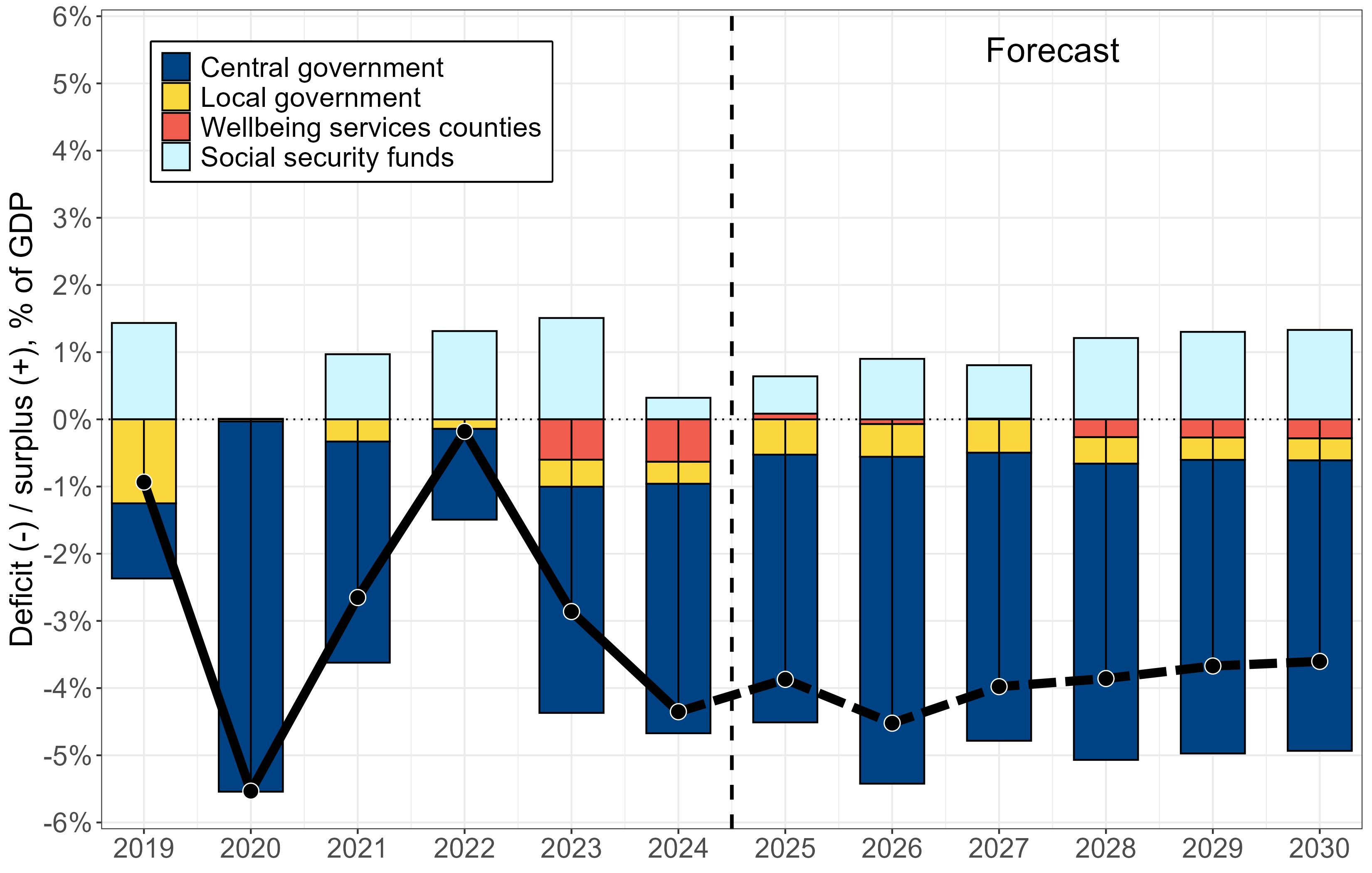
Source: Statistics Finland, Ministry of Finance (2025f).
Part of the current deficit is attributable to the weak cyclical position. However, in the Ministry of Finance forecast, the structural deficit—that is, the deficit independent of the business cycle—is estimated to have been 2.4 per cent of GDP in 2025 and is projected to increase in the coming years.
The bulk of the overall general government deficit is accounted for by the central government deficit. The central government deficit was forecast at 4 per cent of GDP in 2025 and 4.9 per cent in 2026. The increase from 2025 to 2026 reflects not only the recording of fighter jet procurement expenditure but also the tax cut decisions made in spring 2025. The aforementioned policy to increase defence spending also widens the deficit over the forecast years. Defence expenditure is assumed in the forecast to rise to approximately 3 per cent of GDP by the end of the decade. In euro terms, this represents an increase of approximately EUR 3 billion compared to earlier estimates (Ministry of Finance, 2025c).
The central government deficit has been increased by the growth of interest expenditure, driven by both the rise in interest rates and the increase in debt. In the early part of the decade, central government interest expenditure stood at approximately 0.5 per cent of GDP according to Statistics Finland. In 2025, it was forecast at approximately 1.3 per cent of GDP (Ministry of Finance, 2025f). Nearly one percentage point of the increase in the general government deficit as a share of GDP is thus attributable to the rise in central government interest expenditure.
As noted in Chapter 3, the finances of the wellbeing services counties were forecast to have turned to a slight aggregate surplus (0.1 per cent of GDP) in 2025, having been clearly in deficit overall in the two preceding years.26 In the Ministry of Finance forecast, WSC finances are narrowly in balance or slightly in deficit in 2026 and 2027, and return to a more significant deficit in 2028. The forecast takes into account, among other things, pay increases in the health and social services sector, but does not include the counties’ own consolidation measures for 2027 and 2028. If the counties were, however, to aim to cover their accumulated deficits by 2028, the aggregate financial position of the WSCs would be stronger than forecast in 2026–2028. In addition, the counties’ own consolidation measures would improve the central government’s fiscal position with a lag through a lower ex-post adjustment of funding. This would strengthen the overall general government fiscal position compared to the forecast.
The local government deficit widened in 2025 from the previous year according to the Ministry of Finance forecast, reaching 0.5 per cent of GDP. Social security funds have remained in surplus owing to the surplus of the earnings-related pension institutions. The surplus of the earnings-related pension institutions reflects the fact that the earnings-related pension system is a partially funded system. Pension funds generally need to grow in line with pension liabilities to prevent the funding ratio from declining. The surplus of the earnings-related pension institutions is therefore not, as a starting point, a genuine surplus in the same sense as, for example, a possible central government surplus would be, from the perspective of pension financing or public finances as a whole.
Debt ratio
Figure 6.2.2 presents the general government debt ratio in selected countries. At the beginning of the decade, debt ratios rose in all of these countries as a consequence of the pandemic, as economies contracted and public deficits increased. With the exception of Finland, the general government debt-to-GDP ratio has, however, declined from 2020 to 2024 in all the other countries shown in the figure.
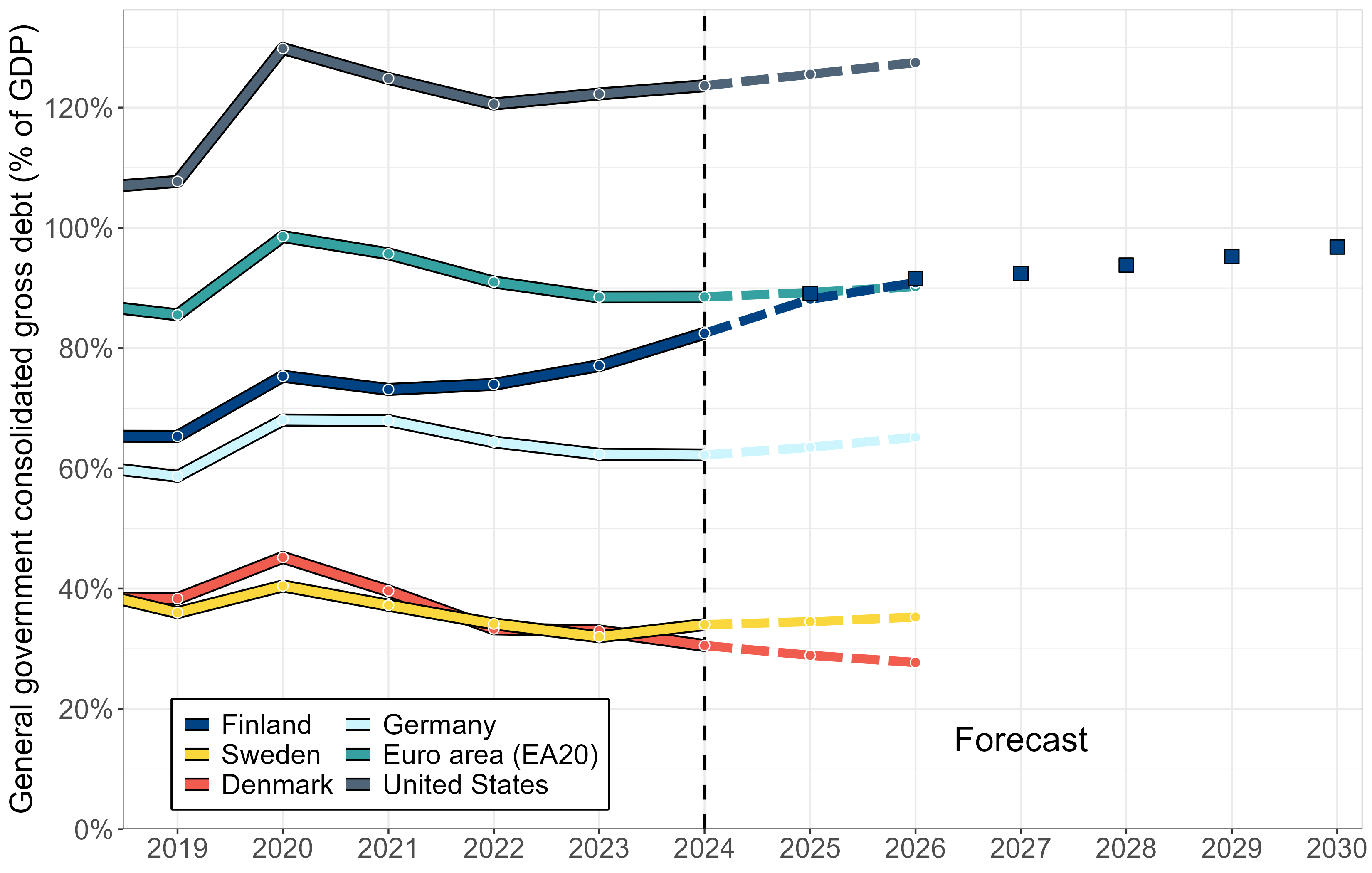
Source: European Commission (AMECO), Ministry of Finance (2025f).
Note: The Ministry of Finance forecasts for Finland’s debt ratio are shown as squares.
According to the Ministry of Finance forecast, Finland’s debt ratio rose to 89.1 per cent in 2025, compared to somewhat below 80 per cent in 2020 and approximately 65 per cent in 2019 (Ministry of Finance, 2025f). According to the forecast, Finland’s debt ratio had risen by 2025 to roughly the same level as the euro area average. Just five years earlier, Finland’s debt ratio was approximately 20 percentage points below the euro area average. At the same time, Finland’s debt ratio has risen significantly above those of its Nordic peers, such as Sweden and Denmark.
According to the Ministry of Finance’s latest winter 2025 forecast, the growth in the debt ratio will not level off in line with the government programme target at the end of the government term, not even momentarily, although certain measures by the government, such as the additional withdrawal from the State Pension Fund discussed above, temporarily reduce borrowing in 2027. It should, of course, be noted that public finance forecasts are subject to various uncertainties beyond cyclical developments, such as the pace at which WSC finances return to balance or the extent to which income tax cuts are ultimately reflected in tax revenues in the short and long term. Nevertheless, on the basis of the Ministry of Finance’s most recent forecast, achieving the debt ratio target would appear to require either new, rapidly effective measures or stronger-than-expected cyclical conditions in the near term.
Developments in public finances from the perspective of EU fiscal rules
Under the EU fiscal rules, the general government deficit should not exceed 3 per cent and debt should not exceed 60 per cent of GDP. In the preventive arm of the rules, so-called net expenditure paths are now also monitored alongside the deficit.27 Each member state has committed to complying with a net expenditure path endorsed by the Council of the European Union, which should satisfy the numerical conditions derived from the debt sustainability analysis and the safeguard clauses of the rules. Significant deviations from the agreed net expenditure path may lead to an excessive deficit procedure. The Council of the European Union endorsed Finland’s medium-term plan and its net expenditure path in January 2025 (Council of the European Union, 2025a).
In spring 2025, however, flexibility was introduced into the EU rules, motivated by the need to increase defence spending. In March, the European Commission proposed a coordinated activation of national escape clauses, allowing greater net expenditure growth and/or general government deficits than would normally be permitted when member states increase their defence spending (European Commission, 2025a).
While the escape clause is in force, the European Commission and the Council of the European Union may refrain from establishing the existence of an excessive deficit if the breach of the 3 per cent deficit reference value (a breach of the deficit criterion) or non-compliance with the net expenditure path (a breach of the debt criterion) is attributable to the increase in defence spending. The maximum amount of flexibility is 1.5 per cent of GDP, and the reference year for defence spending is 2021, i.e. the situation before Russia’s full-scale invasion of Ukraine. In other words, the 3 per cent deficit reference value (relative to GDP) could be exceeded under the flexibility provisions during 2025–2028 by the amount by which the GDP share of defence spending has increased since 2021, but by no more than 1.5 per cent of GDP.
With regard to the net expenditure path, the flexibility introduced into the rules also operates in another way: following the activation of the escape clause, the maximum permissible net expenditure growth is calculated, unlike in the original net expenditure path, without applying the safeguard clauses contained in the rules. In Finland’s case, disregarding the effect of the safeguard clauses would have permitted higher net expenditure growth than the original path, as the so-called debt sustainability safeguard was the most binding constraint on net expenditure growth when Finland’s original net expenditure path was determined. With regard to net expenditure, the ceiling on flexibility related to the growth of defence spending (1.5 per cent of GDP) applies when deviations from the net expenditure path are recorded on the so-called extended control account.28
Finland applied for the activation of the national escape clause from the EU at the end of April, and the activation was approved for Finland in summer 2025.29 The national escape clause covers the years 2025–2028.
The European Commission assesses compliance with the rules twice a year. Based on the realised deficit in 2024 and the forecast deficit for 2025, Finland would likely have been subject to an excessive deficit procedure as early as spring 2025 without the exceptions introduced into the rules. However, the Commission did not yet recommend opening an excessive deficit procedure in June 2025, citing the activation of the escape clause and Finland’s increased defence spending (European Commission, 2025c).
In late 2025, however, the Commission proposed placing Finland in the excessive deficit procedure, as it assessed that Finland was breaching the deficit criterion even when the increase in defence spending under the escape clause was taken into account (European Commission, 2025b). The Council of the European Union formally decided to open the procedure in January 2026. As a consequence of the opening of the excessive deficit procedure, a corrective net expenditure path is proposed for Finland, which thus replaces the previous net expenditure path. The corrective net expenditure path is based on the minimum adjustment required under EU legislation, according to which the structural primary balance should improve annually by 0.5 percentage points relative to GDP. The objective of the Commission’s recommendation is that Finland’s deficit should be below 3 per cent of GDP in 2028.
The proposed corrective net expenditure path is shown on the second-to-last row of Table 6.2.1. According to this path, net expenditure could grow by an average of approximately 1.5 per cent per year until 2028, which is clearly a slower rate of growth than the original net expenditure path or the maximum permissible net expenditure growth under the escape clause. According to the Ministry of Finance forecast shown on the bottom row of the table, net expenditure declined by 0.1 per cent in 2025. This reflects, among other things, the increase in value-added taxation implemented in autumn 2024, as tax increases reduce net expenditure in the same manner as spending cuts. According to the forecast, however, net expenditure is projected to grow significantly faster than the corrective net expenditure path in 2026–2028.
|
| 2025 | 2026 | 2027 | 2028 | |
| Original net expenditure path endorsed by the Council of the European Union | 1.6 | 1.9 | 2.6 | 2.6 | |
| Maximum increase in net expenditure after the removal of safeguards (escape clause) | 2.6 | 2.7 | 2.7 | 2.8 | |
| Corrective net expenditure path (EDP) | 1.3 | 1.5 | 1.8 | ||
| Change in net expenditure (MoF forecast) | \(-\)0.1 | 4.0 | 2.3 | 3.3 | |
Sources: Council of the European Union (2025a,b), European Commission (2025b), Ministry of Finance (2025f,g).
The increase in defence spending can, however, still be taken into account when assessing compliance with the net expenditure path. This provides Finland with flexibility regarding net expenditure growth going forward as well.30 The extent of the flexibility ultimately provided by the defence spending exception clause remains somewhat unclear, as the Commission, which monitors compliance with the rules, may exercise discretion in its overall assessments. It is clear, however, that the spring 2025 tax cut decisions will at the very least not make it easier for Finland to remain on the net expenditure path set for it.
6.3 Fiscal stance
Many of the consolidation measures decided by the government took effect in 2025, tightening fiscal policy by an estimated EUR 3 billion compared to the previous year (Ministry of Finance, 2025c). At the same time, changes in social security contributions strengthened public finances in 2025 by just over EUR 600 million compared to the previous year, when the impact of contribution changes on tax revenue and public sector employer contributions is also taken into account (Ministry of Finance, 2025c). Taken together, this means that, as the sum of discretionary policy measures and changes in social security contributions, fiscal policy tightened by approximately 1.3 per cent of GDP in 2025.31
The fiscal consolidation taking effect in 2025 is also reflected in Figure 6.3.1 as a change in the structural primary balance from \(-\)1.5 per cent to \(-\)0.7 per cent between 2024 and 2025. The structural primary balance is defined as the cyclically adjusted fiscal position net of interest expenditure and one-off measures. It is intended to represent the primary balance—that is, the deficit excluding interest expenditure—that would be achieved under normal cyclical conditions.
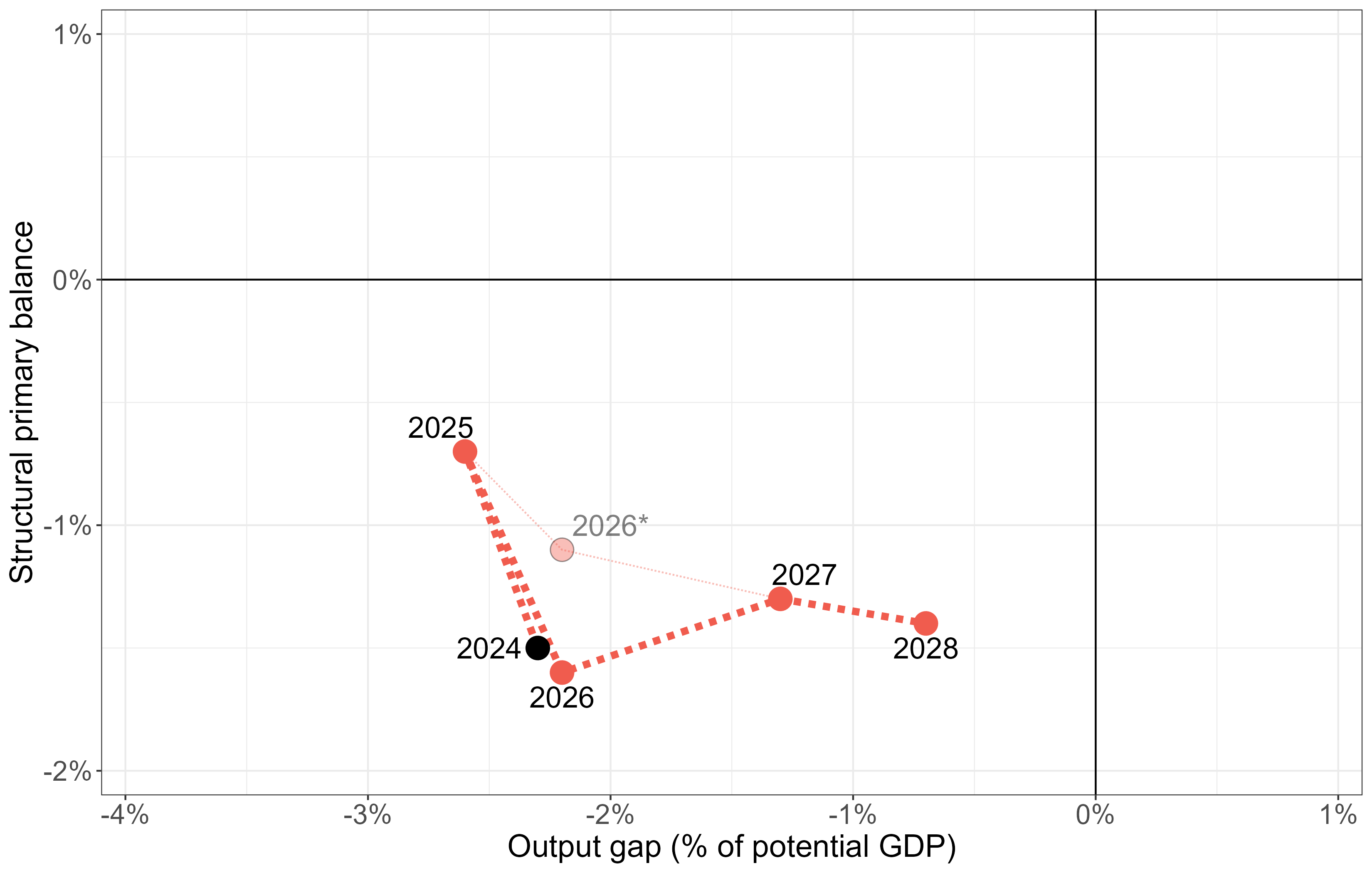
Source: Ministry of Finance (2025f), Council’s calculations.
Note: The shaded dot (2026*) represents the structural primary balance excluding the estimated 0.5 per cent
deficit-deepening effect of fighter jet deliveries in 2026.
Unlike discretionary policy measures, the change in the structural primary balance also captures changes affecting public finances that are not the result of new government decisions, such as the increase in expenditure due to population ageing. Measuring the structural deficit relies, in addition to the deficit forecast, on model-based estimates of the output gap and assumptions about the effects of cyclical fluctuations on public finances, both of which involve uncertainties. The fiscal tightening implied by the structural primary balance may therefore differ considerably from the picture given by the sum of discretionary policy measures.
Fiscal policy tightened in 2025 on both measures compared to the previous year. However, the tightening appears significantly smaller when measured by the change in the structural deficit than by discretionary policy measures. This is likely explained in part by the fact that public expenditure tends to grow even without new decisions, for example as a result of population ageing. Such structural expenditure growth, which the structural deficit seeks to capture, offsets the negative impact of discretionary consolidation measures on aggregate demand.
The fiscal tightening in 2025 coincided with a rather weak cyclical position. Based on Figure 6.3.1, the economy was 2.6 per cent below potential as measured by the output gap in 2025. Potential output is typically defined as the maximum level of output that the economy can sustain without accelerating inflation. A clearly negative output gap is consistent with, for example, the rapid rise in unemployment. On the other hand, the employment rate has nevertheless remained at a relatively high level (see Chapter 2). Based on standard fiscal policy multipliers related to aggregate demand and the change in the structural deficit, the negative impact of fiscal tightening on economic growth in 2025 was of the order of one percentage point.
On the other hand, according to the Ministry of Finance forecast, the cyclical position as measured by the output gap is broadly similar in 2024, 2025, and 2026. It is therefore not clear that the government could have timed the fiscal tightening significantly better than what actually occurred.
Looking at 2026, the overall package of discretionary measures does not appear to entail any significant fiscal tightening. The consolidation measures on the expenditure side, both those set out in the government programme and those decided subsequently, have a tightening effect. Certain tax increases and changes in social security contributions also work in the same direction. On the other hand, income tax cuts in particular loosen fiscal policy (see Chapter 5). As the sum of these offsetting individual discretionary policy measures and changes in social security contributions, the fiscal stance does not appear likely to change significantly from 2025. This supports economic growth and employment compared to the previous year, when fiscal policy tightened.
As measured by the change in the structural primary balance presented in Figure 6.3.1, fiscal policy is in fact loosening, as the primary balance clearly weakens from 2025 to 2026 in the figure. However, the 2026 data point is affected by the assumption that fighter jet deliveries will have a deficit-deepening impact of approximately 0.5 per cent in the general government deficit as measured in national accounts. The recording of fighter jet procurement in national accounts figures does not, however, reflect a change in fiscal policy that would be significant from the perspective of aggregate demand. The shaded dot (2026*) added to the figure represents the level of the structural primary balance excluding the item related to fighter jet deliveries. Even on this basis, fiscal policy is set to loosen in 2026 compared to the previous year, but only by the order of 0.5 per cent of GDP.
In the years beyond 2026, the structural primary balance is forecast to weaken while output approaches its potential level. New consolidation measures may, on the other hand, once again reduce output relative to potential output by contracting aggregate demand. For the near-term economic outlook, the key question is to what extent growth in net exports offsets the negative impact of spending cuts or tax increases on aggregate demand. Over the longer term, output and employment can grow on the back of exports even if tight fiscal policy contracts domestic demand. However, the reallocation of labour from the domestic sector to export industries takes time. Improvements in output and employment through stronger exports also require sufficiently good competitiveness in export industries. In the short term, this is closely linked to wage developments.32
6.4 Reform of the fiscal policy act
Under the national fiscal policy act (869/2012) that was in force until the end of 2025, the binding fiscal policy rule for Finland was defined in terms of the structural balance. Finland had committed to targeting a structural balance of at least \(-\)0.5 per cent of GDP. The new EU fiscal rules entered into force on 1 April 2025, and the national fiscal policy legislation was reformed accordingly. Finland’s new fiscal policy act (1441/2025) entered into force on 1 January 2026.
Under the new act, the objective of the management of public finances is to ensure that general government debt relative to GDP does not exceed 60 per cent and, over the (very) long term, does not exceed 40 per cent. The actual fiscal policy rule, however, does not concern the debt ratio but rather the combined fiscal position of central and local government, i.e. the difference between their expenditure and revenue. The government sets both a cross-term target and a government-term target for this fiscal position. These targets must be consistent with Finland’s compliance with the EU fiscal rules and with an average annual reduction of the public debt ratio by at least 0.75 percentage points over an eight-year assessment period.
The setting of both the government-term and the cross-term targets is prepared by a parliamentary working group. This may improve cross-party commitment to the objective of consolidating public finances, for instance by facilitating the development of a shared assessment of the fiscal situation. It is, however, likely that the parliamentary group will have very little room for manoeuvre in setting the targets, at least in the near term, as the EU fiscal framework already imposes quite stringent requirements on Finland’s fiscal policy.
The specific measures to achieve the fiscal position targets are always decided by the government in office at the time. The government must review the adequacy of its measures annually in the general government fiscal plan and in the preparation of the central government budget.
The achievement of the fiscal position target is supported by a correction mechanism. From 1 January 2026, the Economic Policy Council serves as the independent fiscal institution required under EU regulation, monitoring compliance with the fiscal policy act. If, in the Council’s overall assessment, the government-term fiscal position target is not on track to be achieved, and there are no acceptable grounds for deviating from the target, the Council will present to the government an assessment of the scale and timing of the corrective measures required. The overall assessment may take into account, for example, the cyclical position.
In addition to monitoring compliance with the fiscal policy rule, the Economic Policy Council will henceforth endorse the macroeconomic forecasts prepared by the Economics Department of the Ministry of Finance twice a year.
The act includes transitional periods for the entry into force of its various provisions. The parliamentary working group will set the first cross-term target in early 2026 for the period 2027–2033. The next government will set the government-term fiscal position target for the final year of the 2027–2031 term. Under the transitional provision of the act, the first fiscal position targets, to be set in 2027, will be set solely on the basis of obligations arising from EU legislation. All provisions of the act will be fully in force only in 2033.
6.5 Council views
The government does not appear to be on track to achieve its key objectives for strengthening public finances during the current government term. According to forecasts, the growth of the debt-to-GDP ratio will not turn as envisaged in the government programme, and the general government deficit in particular is likely to remain clearly larger than the target set out in the programme.
One key reason for falling short of the targets is that some of the consolidation measures included in the government programme were uncertain in their effects from the outset. For example, the government is pursuing significant spending cuts through productivity-enhancing measures in the wellbeing services counties, even though it is in practice difficult to verify whether such improvements actually translate into savings for public finances.
A second reason is that the economic cycle has been somewhat weaker than anticipated. This has directly increased the deficit and has also likely significantly diminished the impact of the measures in the government programme aimed at raising the employment rate.
The strengthening of public finances has also been hampered by the growth of defence expenditure and interest expenditure associated with servicing public debt. In addition, the government has decided on new tax cuts for the latter part of the government term. As a result, fiscal policy is not set to tighten significantly in 2026 compared to 2025. This supports the economic recovery towards the end of the government term. At the same time, however, the tax cuts are likely to weaken public finances.
The government’s discretionary measures taken as a whole are nevertheless clearly strengthening public finances compared to a scenario without them. Their effect in reducing the annual deficit can also be expected to grow over time, as it takes time for the economy to adjust to the weakening of domestic demand caused by consolidation measures.
The outlook for public finances also includes positive factors. Increased household savings and labour force growth may support economic growth and the strengthening of public finances in the near term. Nevertheless, balancing public finances and meeting the requirements set by the EU fiscal rules will require significant new consolidation measures in future government terms.
References